Oil price in 2012-2013

This is a revision to our oil price prediction as based on the difference between the overall PPI and the index of crude oil. Figure 1 compares our previous prediction in May 2011 with actual oil price in 2011 and 2012. In August 2011, the predicted price was a bit higher than the measured one. We expected the price to fall by approximately $5 per month to the level of ~$70 by December 2011. In reality, the price reflected from the high bound of the expected price (dashed line) and grew during the end of 2011. This effect reflects the high level of price volatility during short time intervals. Since February 2012, the price has been returning to the expected price range which expresses the slow fall through 2016, with the uncertainty bounds for the long-term trend in oil price shown in Figure 1. The level of oil price in 2016 is expected between $30 and $60 per barrel.

Here we confirm the oil price trend and its bounds. Red squares show our prediction of oil price through February 2013. Despite local fluctuations, the trend is negative and will bring the price to $45 (±$15) per barrel in 2016.  

Figure 1. The evolution of oil price since 2001 as estimated from the differnce of the overall PPI and the PPI of crude petroleum.

Halliburton's shares

We have already presented updated pricing models for ConocoPhillips and ExxonMobil as based on the differences between CPI and PPI components. Our share pricing concept was introduced two years ago and predicted share prices for a few energy companies. ConocoPhillips (COP) and Exxon Mobil (XOM) from the S&P 500 list were the biggest and demonstrated almost no difference in the sensitivity to the difference between the core and headline CPIs. Halliburton’s share (HAL) was also modeled showed a dramatically different sensitivity. We made a tentative conclusion that COP and XOM might have a larger return to an investor considering energy stocks.

Basically, we demonstrated that the time history of a share price, p(t), (for example, HAL) could be accurately approximated by a linear function of the difference between the core CPI, cCPI(t), and the headline CPI in the United States. At the initial stage of our research, this difference was found to be the best to predict share prices in the energy subcategory.

Mathematically, a share price, HAL(t), (we use a monthly closing price adjusted for dividends and splits) can be approximated by a linear function of the lagged difference between the core and headline CPI:

HAL(t) = A + BdCPI(t+t₁)                                       (1)

where dCPI(t+t₁)=cCPI(t+t₁)–CPI(t+t₁), A and B are empirical constants. In the original model for HAL for the period between 1999 and 2009, A=43, B=-3.5; t is the elapsed time; and t₁=0 year is the time delay between the share and the CPI change, i.e. the CPI has a lag behind the share price.

In this article, we test several pricing models for Halliburton, HAL(t), with the same CPI and PPI components tested for ConocoPhillips and ExxonMobil. The set of defining indices includes: the core and headline CPI, the consumer price index of energy, eCPI, and the producer price index of crude petroleum, pPPI, together with the overall PPI. Thus, we test model (1) for HAL(t) using two different differences for the period between 2001 and 2011: 

HAL(t) = A1 + B1(cCPI(t) - eCPI(t))  (2)   

HAL(t) = A2 + B2(pPPI(t) - PPI(t))         (3) 

All coefficients in (1)-(3) were estimates by the least squares for the period between January 2001 and July 2011. As for ConocoPhillips and ExxonMobil, we found no time delay between the share price and defining differences, i.e. t₁=0. 

Figures 1 through 3 compare three HAL models. Corresponding coefficients are given in Figure captions. As in our original study, the best model (in sense of RMS residual, s) for the period between 2001 and July 2011 is based on the core and headline CPI (s=$4.18). Almost the same accuracy is associated with the model based on the core and energy CPI (s=$4.44).

At the same time, model (3) based on the producer price indices is the worst (s=$9.31). This may mean that Halliburton does not depend much on the producer price indices. Interestingly, the change in oil price does accurately describe the period of the financial crisis. However, the model fails to predict slow changes in the share price. Currently, the deviation between the observed and predicted prices is $20.

Halliburton’s shares were less sensitive to the change in consumer prices during the financial crisis than those of XOM and COP. However, the overall agreement between the observed and predicted prices is very good for the past ten years. One can expect that the current deviation from the predicted price will disappear in the near future and the observed price will fall down to $40 per share. In the long-run, the expected fall in oil price at a five-year horizon down to $30 per barrel will likely result in a proportional decrease in HAL’s shares.

Figure 1.  The observed HAL price and that predicted from the core and headline CPI.  A=$43, B=-3.4.

Figure 2.  The observed HAL price and that predicted from the core CPI and the consumer price index of energy.  A1=$30, B1=-0.3.

Figure 3.  The observed HAL price and that predicted from the overall PPI and the producer price index of crude petroleum (domestic production).  A2=$25, B2=-0.13. 

Share prices: ExxonMobil vs ConocoPhillips

In a previous post we have extended our original pricing model for ConocoPhillips and found that the evolution of its share can be best approximated by a linear function of the difference between the core CPI, coreCPI, and the consumer price index of energy, eCPI.  Originally, the model for a share price, p(t), (we use a monthly closing price adjusted for dividends and splits) was based on the difference between the core and headline CPI:

p(t) = A + B (coreCPI - CPI(t))                                 (1)

where A and B are empirical constants; t is the elapsed time.  

Here we test pricing models for ExxonMobil, XOM(t), with the same CPI and PPI components as we used for ConocoPhillips. The set of defining indices includes the core and headline CPI, the consumer price index of energy, eCPI, and the producer price index of crude petroleum, pPPI, together with the overall PPI. Thus, we test model (1) with p(t)=XOM(t) and two different models for the period between 2001 and 2011: 

XOM(t) = A1 + B1(coreCPI - eCPI(t))  (2) 

XOM(t) = A2 + B2(pPPI - PPI(t))         (3) 

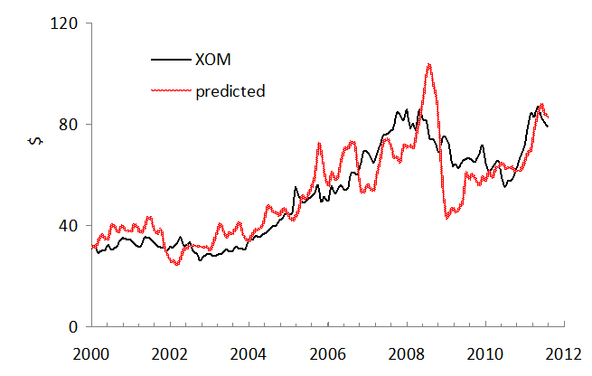
Figures 1 through 3 compare three XOM models. Coefficients in (1) through (3) are given in corresponding Figure captions. The best model (in sense of RMS residual, s) for the period between 2001 and July 2011 is based on the core and headline CPI (s=$9.32). Almost the same accuracy is associated with the model based on the core and energy CPI (s=$9.84). At the same time, model (3) based on the producer price indices is the worst (s=$10.9).

There is a dramatic difference between ExxonMobil and ConocoPhillips. The former company was less sensitive to the change in consumer prices during the financial crisis. The predicted amplitude is much higher than that observed between 2008 and 2009. ConocoPhillips has followed up the change in the difference between the core and energy CPI. When the behavior between 2008 and 2009 is extrapolated into the 2010s, the expected fall in oil price at a five-year horizon down to $30 per barrel will likely not result in a proportional decrease of XOM’s shares.

Figure 1.  The observed XOM price and that predicted from the core and headline CPI.  A=$86, B=-5.8.

Figure 2.  The observed XOM price and that predicted from the core CPI and the consumer price index of energy.  A1=$56, B1=-0.27.

Figure 3.  The observed XOM price and that predicted from the overall PPI and the producer price index of crude petroleum (domestic production).  A2=$68, B2=-0.55. 

ConocoPhillips share price to fall

Our original pricing model states that a share price, for example, that of ConocoPhillips, COP(t), can be approximated by a linear function of the difference between the core CPI, coreCPI, and headline CPI:

COP(t) = A + B (coreCPI - CPI(t))                          (1)

where A and B are empirical constants; t is the elapsed time.  Here we extend the set of defining indices by the consumer price index of energy, eCPI, and the producer price index of crude petroleum, pPPI, together with the overall PPI. Thus, we test the following models for the period between 2001 and 2011:

COP(t) = A1 + B1(coreCPI - eCPI(t))  (2)   

COP(t) = A2 + B2(pPPI - PPI(t))         (3) 

Figures 1 through 3 compare the original and new predictions for COP. Coefficients in (1) through (3) are given in Figure captions. The best model for the period between 2001 and July 2011 is based on the index of energy and core CPI. Practically the same accuracy is associated with the original model as based on the core and headline CPI. At the same time, model (3) based on the producer price indices is the worst and has failed to predict the amplitude of the largest oscillation in 2008.  

We have predicted oil price to fall through 2016. In 2011, we expect oil price to fall down to $70 per barrel. Considering these short- and mid-term predictions one can conclude that ConocoPhillips share price will be falling as well. 

Figure 1.  The observed COP price and that predicted from the core and headline CPI.  A=75, B=-5.5.

Figure 2.  The observed COP price and that predicted from the core CPI and the consumer price index of energy.  A1=58, B1=-0.54.

Figure 3.  The observed COP price and that predicted from the overall PPI and the producer price index of crude petroleum (domestic production).  A2=45, B2=-0.3.

Shimmy in economic gear. How far is the U.S. economy from a runaway?

Shimmy is a well-known mechanical effect in aircraft landing gear. During landing and take-off, the nose wheel oscillates about the vertical axis, sometimes with increasing amplitude. In the case of severe resonance oscillation, shimmy may result in the wheel  destruction.  Instructively, shimmy usually occurs in a specific band of aircraft velocities.  (A much safer but typical case of shimmy is observed in a shopping trolley.) The shimmy effect is well known and relatively well understood and modelled, although not completely.  

As an economic analogue of shimmy, we propose to take a look at the current oscillations in commodity prices.  Is it actually an economic shimmy? In several figures below we present the evolution of relative prices, pi, of selected commodities, iPPI. In order to remove the base effect we calculate the deviation from the overall PPI, PPI, and normalize it to the PPI:

pi(t)= (PPI-iPPI)/PPI

where i corresponds to iron&steel, gold ores, crude petroleum (domestic production),  copper ores, aluminium base scrap and grain. Four from these six basic commodities demonstrate a clear start of shimmy around 2005.  Aluminium base scrap and grain had higher oscillations in the past, but can be also characterized by an elevated volatility during the past 5 years.

Overall, a higher volatility is not a surprise for the market but since 2005 is has a coherent driving force behind all commodities. It is likely that there is a positive feed back in the loop of commodity pricing with money flooding into the commodity market without any restriction. For a nose wheel, similar mechanical feedback leads to shimmy and aircraft accidents. For the U.S. economy, one can expect a price runaway (gold is a candidate) if the positive feedback observed since 2005 is further retained. How far is the current situation from an accident?

Does crude drive the price index of steel and iron? (update)

We have been following the link between price indices of iron&steel and crude oil (domestic production) since 2009. This is a quarterly update. The previous update included PPI data as of November 2010. Here we extend the set by data available after April 13, 2011. Otherwise, we retain the form of the report untouched.

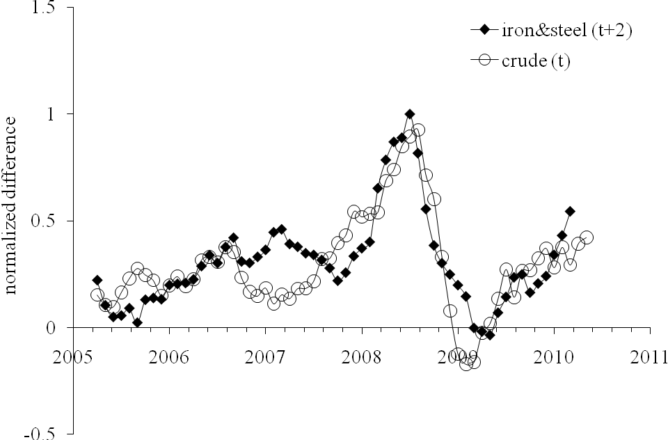
Historically, we first reported that the price index of crude oil had been likely evolving in sync with that of iron and steel, but with a lag of two months in September 2009  [1].  In order to present both indices in a comparable form, the difference between a given index, iPPI (i.e. iron&steel and crude), and the overall PPI was normalized to the PPI: (iPPI(t)-PPI(t))/PPI(t). The normalized differences represent the evolution of the rate of deviation from the PPI over years.  

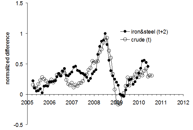
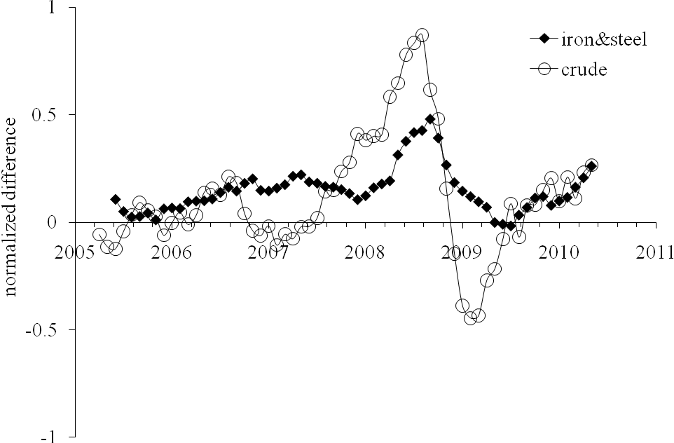
Figure 1 depicts the corresponding time histories of the normalized deviations from the PPI, including the most recent period since December 2010.  Simple visual inspection reveals the following feature: the (normalized deviation from the PPI of the) index of iron and steel lags by approximately two months behind the (normalized) index of crude oil.

Figure 1. The deviation of the iron and steel price index and the index of crude oil from the PPI, normalized to the PPI.

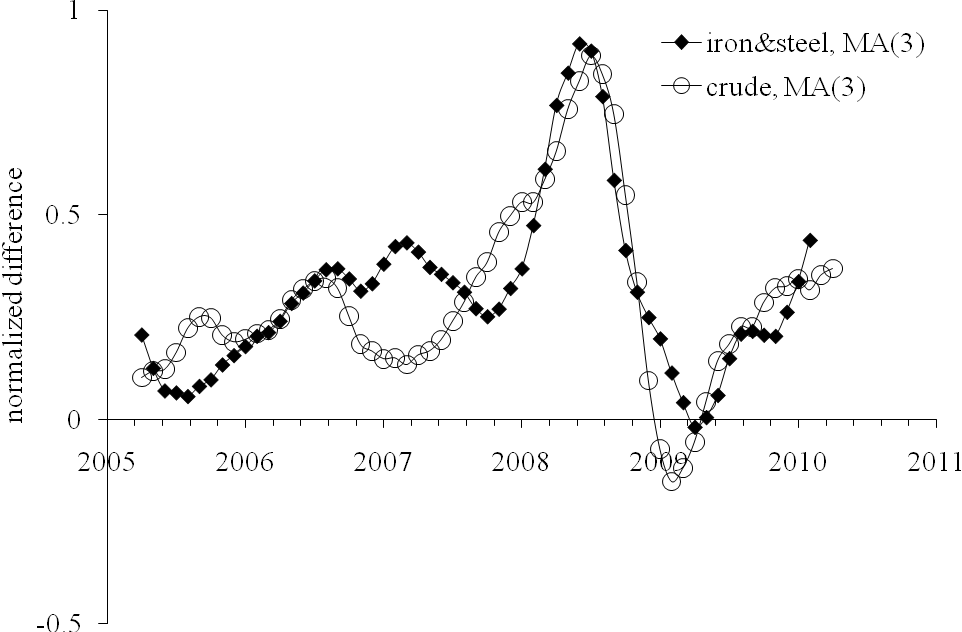
In order to reduce both deviations to the same scale we additionally normalized the curves in Figure 1 to their peak values between 2005 and 2011

(iPPI(t)-PPI(t))/[PPI(t)*max{iPPI-PPI)}]

This scaling allows a direct comparison of corresponding shapes. In Figure 2, we display the normalized index of iron and steel shifted by two months ahead to synchronize its peak with that observed in the normalized index for crude petroleum. The scaled index of crude demonstrates just short-term deviations from the index of iron and steel in the overall shape and timing of the peak and trough. Simple smoothing with MA(3) makes the curves resemblance even better. As an invaluable benefit of the resemblance, one can use the two-month lag to predict the future of the iron and steel price index.

Figure 2. Deviation of the iron and steel price index from the PPI, normalized to the PPI and the peak value after 2005 as compared to the deviations of the index for crude petroleum normalized in the same way. The normalized index for iron and steel is shifted two months ahead.

Conclusion

Between 2006 and 2011, the deviation of the price index of iron and steel from the PPI in the USA repeats the trajectory of the deviation of the index of crude petroleum (domestic production) with a two-month lag. Therefore, the prediction of iron and steel price for at this horizon is a straightforward one.  

References

1. Kitov, I., Kitov, O., (2009). Sustainable trends in producer price indices, Journal of Applied Research in Finance, Spiru Haret University, Faculty of Financial Management and Accounting Craiova, vol. I(1(1)_ Summ), pp. 43-51

Does crude drive the price index of steel and iron?

This update includes the readings of the producer price indexes of crude oil and iron&steel for November 2010.

In September 2009, we reported that the price index of crude oil had been likely evolving in sync with that of iron and steel, but with a lag of two months [1].  In order to present both indexes in a comparable form, the difference between a given index, iPPI, and the overall PPI was normalized to the PPI: (iPPI(t)-PPI(t))/PPI(t). The normalized differences represent the evolution of the rate of deviation from the PPI over years.  

Figure 1 depicts the corresponding time histories of the normalized deviations from the PPI, including the most recent period since June 2010.  Simple visual inspection reveals the following feature: the (normalized deviation from the PPI of the) index of iron and steel lags by two months behind the (normalized) index of crude oil.

Figure 1. The deviation of the iron and steel price index and the index of crude oil from the PPI, normalized to the PPI.

In order to reduce both deviations to the same scale we additionally normalized the curves in Figure 1 to their peak values between 2005 and 2010

(iPPI(t)-PPI(t))/[PPI(t)*max{iPPI-PPI)}]

This scaling allows a direct comparison of corresponding shapes. In Figure 2, we display the normalized index of iron and steel shifted by two months ahead to synchronize its peak with that observed in the normalized index for crude petroleum. The scaled index of crude demonstrates just short-term deviations from the index of iron and steel in the overall shape and timing of the peak and trough. Simple smoothing with MA(3) makes the curves resemblance even better. As an invaluable benefit of the resemblance, one can use the two-month lag to predict the future of the iron and steel price index.

Figure 2. Deviation of the iron and steel price index from the PPI, normalized to the PPI and the peak value after 2005 as compared to the deviations of the index for crude petroleum normalized in the same way. The normalized index for iron and steel is shifted two months ahead.

Conclusion

Between 2006 and 2010, the deviation of the price index of iron and steel from the PPI in the USA repeats the trajectory of the deviation of the index of crude petroleum (domestic production) with a two-month lag. Therefore, the prediction of iron and steel price for at this horizon is a straightforward one.  

References

1. Kitov, I., Kitov, O., (2009). Sustainable trends in producer price indices, Journal of Applied Research in Finance, Spiru Haret University, Faculty of Financial Management and Accounting Craiova, vol. I(1(1)_ Summ), pp. 43-51

Does crude drive the price index of steel and iron?

This is a quarterly update.

In September 2009, we reported that the price index of crude oil had been likely evolving in sync with that of iron and steel, but with a lag of two months. In order to present both indices in a comparable form, the difference between a given index, iPPI, and the overall PPI was normalized to the PPI: (iPPI(t)-PPI(t))/PPI(t). The normalized differences represent the evolution of the rate of deviation from the PPI over years.

Figure 1 depicts the corresponding time histories of the normalized deviations from the PPI, including the most recent period since June 2010. Simple visual inspection reveals the following feature: the (normalized deviation from the PPI of the) index of iron and steel lags by two months behind the (normalized) index of crude oil.

Figure 1. The deviation of the iron and steel price index and the index of crude oil from the PPI, normalized to the PPI.

In order to reduce both deviations to the same scale we additionally normalized the curves in Figure 1 to their peak values between 2005 and 2009:

(iPPI(t)-PPI(t))/[PPI(t)*max{iPPI-PPI)}]

This scaling allows a direct comparison of corresponding shapes. In Figure 2, we display the normalized index of iron and steel shifted by two months ahead to synchronize its peak with that observed in the normalized index for crude petroleum. (The period between May and July 2010 is included.) The scaled index of crude demonstrates just minor discrepancies from the index of iron and steel in the overall shape and timing of the peak and trough. Simple smoothing with MA(3) makes the curves resemblance even better. As an invaluable benefit of the resemblance, one can use the two-month lag to predict the future of the iron and steel price index.

Figure 2. Deviation of the iron and steel price index from the PPI, normalized to the PPI and the peak value after 2005 as compared to the deviations of the index for crude petroleum normalized in the same way. The normalized index for iron and steel is shifted two months ahead.

Conclusion

Between 2006 and 2010, the deviation of the price index of iron and steel from the PPI in the USA repeats the trajectory of the deviation of the index of crude petroleum (domestic production) with a two-month lag. Therefore, the prediction of iron and steel price for at this horizon is a straightforward one. It is likely that in the fourth quarter of 2010 the index of iron and steel will be decreasing following the observed fall in the index for crude petroleum.

References

Kitov, I., Kitov, O., (2009). Sustainable trends in producer price indices, Journal of Applied Research in Finance, Spiru Haret University, Faculty of Financial Management and Accounting Craiova, vol. I(1(1)_ Summ), pp. 43-51

PPI of copper ores and grains

Three months ago we revisited our prediction on the evolution of the PPI of copper and grain, which had been made in 2009. The original prediction limited the level of the copper PPI in 2010:

Therefore, copper price will likely not be growing to its peak in April 2008 (491.7), but will likely return to heights around 350.

Three months ago we suggested that:

In the short-run, the index for copper will NOT be growing too long, at least NOT till the end of 2010.

Figure 1 compares the prediction and actual behavior for the producer price index of copper ores relative to the overall PPI. All in all, the prediction was right: by the end of 20009 the price index of copper has reached the level of 350 (375) and even higher in the beginning of 2010 (443 in April). However, it has not reached the 2008 level and started to fall in the second half of 2010. It is very likely that the fall will continue, potentially with a higher volatility, in 2010 and will be stretched into 2011. At a two to four year horizon, the price index for copper ores should return to the pre-2008 level.

Figure 1. Evolution of the price index of copper ores relative to the PPI.

The price index for grains has been following our predictions as well. In 2009 we wrote:

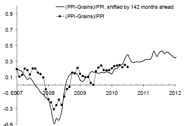
It is instructive to compare two major spikes in the grains index in 1996 and 2008 relative to the PPI. In order to avoid comparing absolute values, which undergo secular growth, the evolution of the difference between the PPI and the price index of grains normalized to the PPI. Figure 3 presents the normalized curves. The left panel shows that the spike in the grains PPI in July 1996 is similar in relative terms to that observed in 2008. The right panel tests this hypothesis: the spikes are synchronized - for the black line is shifted forward by 142 months. From this comparison, it is likely that decline in the grains index relative to the PPI will extend into the 2010s.


Three months ago we confirmed the prediction that the index of grains would follow the path observed in 1996:

The index for grains will continue its decline relative to the PPI. As a consequence, one can expect that the index for food will be also decreasing and this decline will stretch into the 2011

Figure 2 illustrates the accuracy of our prediction of the index of grains. The index has been falling relative to the PPI and the trajectory actually repeats that observed 142 months before. We expect the normalized difference to follow up the once observed recovery path. It is interesting that this time the through was not as deep as in 1996. Supposedly, there are more efficient mechanisms counteracting the growth in the price of grains when were in 1996. Judging from Figure 2, the index of grain will not be growing during the next several years.

Figure 2. Evolution of the difference between the PPI and the price index of grains normalized to the PPI. Upper panel: Comparison of the current curve to that observed 142 months ago. Lower panel: Same as in the upper panel; the most recent period.

Short term prediction

In the short-run, the index for copper will likely be falling in 2010. The index for grains will continue its slight decline relative to the PPI.

For details see also our papers:

 1. Kitov, I., Kitov, O., (2008). Long-Term Linear Trends In Consumer Price Indices, Journal of Applied Economic Sciences, Spiru Haret University, Faculty of Financial Management and Accounting Craiova, vol. 3(2(4)_Summ), pp. 101-112.

2. Kitov, I., (2009). Apples and oranges: relative growth rate of consumer price indices, MPRA Paper 13587, University Library of Munich, Germany.

3. Kitov, I., Kitov, O., (2009). A fair price for motor fuel in the United States, MPRA Paper 15039, University Library of Munich, Germany,

4. Kitov, I., Kitov, O., (2009). Sustainable trends in producer price indices, Journal of Applied Research in Finance, v. 1, (in press)

5. Kitov, I., Kitov, O., (2009). PPI of durable and nondurable goods: 1985-2016, MPRA Paper 15874, University Library of Munich, Germany

6. Kitov, I., (2009). Predicting gold ores price, MPRA Paper 15873, University Library of Munich, Germany

7. Kitov, I., (2009). Predicting the price index for jewelry and jewelry products: 2009-2016, MPRA Paper 15875, University Library of Munich, Germany

Crude in 2010

Three months ago we presented a forecast for the PPI for crude oil and oil price in August 2010. Tentatively, we put the index at the level between 160 and 180 in August 2010. Crude oil price corresponding to this level of index should be between $62 and $70 per barrel. It’s time to revisit the price.

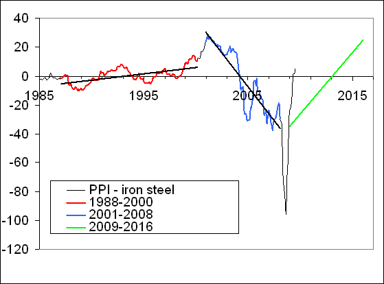
All our estimates are based on the existence of long-term sustainable trends in the differences between various subcategories of the producer price index (PPI). The concept is illustrated in Figure 1, where the difference between the overall PPI and that for crude petroleum is approximated by three linear trends. The most recent trend started in the beginning of 2010 and has been strengthening since then. Without loss of generality, we consider that the new developing trend will be a mirror reflection (opposite but equal slope) of the previous trend observed between 2002 and 20008. This is the long-term prediction for oil price with the PPI of crude at the level of 75 point in 2016.

Figure 2 presents the short term view elaborating on the most recent transition period from July 2008 to August 2009 and the details of the new trend. In March 2009, we presented two predictions. In (1) we presumed that, when reached the trend, the price would follow along it. Second prediction was based on a “dynamic overshoot” with oil price dropping much below the new trend, as shown by solid diamonds in Figure 2. From these two predictions, the first was right.

Figure 3 details our prediction made in June 2010 on the evolution of the oil price index between June and August 2010. We expected that the price would fall and the predicted curve rise above the trend, as shown by red circles. This is a consequence of the fluctuation around the trend: the price can not be retained just on one side of the trend line. The measured price did not touch the trend line, however. So, our prediction was not fully right despite the price actually has fallen significantly. The Augusts’ estimates of the producer price index for crude petroleum will be published in the middle of September. It will definitely show a decrease relative to July, but the price will not drop to $70 per barrel.

Therefore, we foresee two possible scenarios. A more likely one supposes that the price in September will fall below $70 per barrel and the measured difference (open circles) in Figure 3 will intercept the trend line. This scenario will be in line with our prediction of the S&P 500 level below 1000 in September.

We can not exclude that the price (and the S&P 500) will not drop in September cumulating more potential relative to the trends. Then, this must happen in October-November and the potential drop will just increase in time as the deviation between the actual curve and the trend. The trend itself seems to be well-established already since the price goes along the trend since August 2009. It might also happen that the true trend is different form the predicted one. It may have lower slope than during the previous period. Then the price will be decreasing a lower rate into the second half of the 2000s. One can better estimate the trend slope in couple years, but before actual data are available we will retain our hypothesis on the slope value.

All in all, we expect the price index of crude petroleum to follow the new trend in the long run with short-term fluctuations of various amplitude and period.

Figure 1. Sustainable linear trends in the difference between the overall PPI and that for crude oil between 1987 and 2010. Currently, we observe the emergence of a new trend, which supposedly is a mirror reflection of the previous one.

Figure 2. The evolution of the difference between the overall (all commodities) PPI and that for crude oil.

Figure 3. The measured and predicted difference between the overall PPI and the index for crude petroleum.

1. Crude Oil And Motor Fuel: Fair Price Revisited

Does crude drive the price index of steel and iron?

In September 2009, we reported that the price index of crude oil had been likely evolving in sync with that of iron and steel, but with a lag of two months. In order to present both indices in a comparable form, the difference between a given index, iPPI, and the overall PPI was normalized to the PPI: (iPPI(t)-PPI(t))/PPI(t). The normalized differences represent the evolution of the rate of deviation from the PPI over years.

Figure 1 depicts corresponding time histories of the normalized deviations from the PPI. Simple visual inspection reveals the following feature: the (normalized deviation from the PPI of the) index of iron and steel lags by two months behind the (normalized) index of crude oil.

Figure 1. The deviation of the iron and steel price index and the index of crude oil from the PPI, normalized to the PPI.

In order to reduce both deviations to the same scale we additionally normalized the curves in Figure 1 to their peak values between 2005 and 2009:

(iPPI(t)-PPI(t))/[PPI(t)*max{iPPI-PPI)}]

This scaling allows a direct comparison of corresponding shapes. In Figure 2, we display the normalized index of iron and steel shifted by two months ahead to synchronize its peak with that observed in the normalized index for crude petroleum. The scaled index of crude demonstrates just minor discrepancies from the index of iron and steel in the overall shape and timing of the peak and trough. Simple smoothing with MA(3) makes the curves resemblance even better. As an invaluable benefit of the resemblance, one can use the two-month lag to predict the future of the iron and steel price index.

Figure 2. Deviation of the iron and steel price index from the PPI, normalized to the PPI and the peak value after 2005 as compared to the deviations of the index for crude petroleum normalized in the same way. The normalized index for iron and steel is shifted two months ahead.

Conclusion

Between 2006 and 2010, the deviation of the price index of iron and steel from the PPI in the USA repeats the trajectory of the deviation of the index of crude petroleum (domestic production) with a two-month lag. Therefore, the prediction of iron and steel price for at this horizon is a straightforward one. It is likely that in 2010 the index of iron and steel will approach closely the level attained in August 2008. From this level, it will be declining in the long run following the new trend of oil price, as shown in our previous post.

References

Kitov, I., Kitov, O., (2009). Sustainable trends in producer price indices, Journal of Applied Research in Finance, Spiru Haret University, Faculty of Financial Management and Accounting Craiova, vol. I(1(1)_ Summ), pp. 43-51

Copper ores and grains. A year after

About a year ago we published a prediction for copper and grain:

Therefore, copper price will likely not be growing to its peak in April 2008 (491.7), but will likely return to heights around 350.

In the short-run, the index for copper will be growing at least till the end of 2009. The index for grains will continue its decline relative to the PPI. As a consequence, one can expect that the index for food will be also decreasing and this decline will stretch into the 2010s.

Figure 1 compares the prediction and actual behavior for the producer price index of copper ores relative to the overall PPI. All in all, the prediction was right: by the end of 20009 the price index of copper has reached the level of 350 (375) and even higher in the beginning of 2010 (443 in April). However, it has not reached the 2008 level. It is difficult to foresee further evolution, but one cannot exclude the price to grow beyond that in 2008.

Figure 2 illustrates the accuracy of our prediction of the index of grains. The index has been falling relative to the PPI and the trajectory actually repeats that observed 142 months before, as explained the previous post:

It is instructive to compare two major spikes in the grains index in 1996 and 2008 relative to the PPI. In order to avoid comparing absolute values, which undergo secular growth, the evolution of the difference between the PPI and the price index of grains normalized to the PPI. Figure 3 presents the normalized curves. The left panel shows that the spike in the grains PPI in July 1996 is similar in relative terms to that observed in 2008. The right panel tests this hypothesis: the spikes are synchronized - for the black line is shifted forward by 142 months. From this comparison, it is likely that decline in the grains index relative to the PPI will extend into the 2010s.

Figure 1. Evolution of the price index of copper ores relative to the PPI. Upper panel: September 2009. Lower panel: April 2010.

Figure 2. Evolution of the difference between the PPI and the price index of grains normalized to the PPI. Left panel: September 2009. Right panel: April 2010.

Short term prediction

In the short-run, the index for copper will NOT be growing too long, at least NOT till the end of 2010. The index for grains will continue its decline relative to the PPI. As a consequence, one can expect that the index for food will be also decreasing and this decline will stretch into the 2011.

We can also repeat the conclusion from the post one year ago

In the long run, the producer price index for copper and that of grains both demonstrate practically unpredictable behavior with unclear future. This observation only emphasizes the importance of sustainable trends observed for other commodities. In the US economy, as in many natural systems, there exist trend components, oscillating components, and random components.

PPI of metals: annual revision

About a year ago we revised the evolution of several price indices of metals. Our general approach is based on the presence of long-term sustainable trends in the evolution of the CPI and PPI in the United States. The difference between various components of these indices is not a random but rather a predetermined process, as shown in a series of papers we published in 2008-2009 [1-4]. Using these trends, one can predict consumer and producer price indices for select goods, services and commodities [5-7]. We have summarized these papers and some more studies in a monograph “Deterministic mechanics of pricing” published by LAP [8].

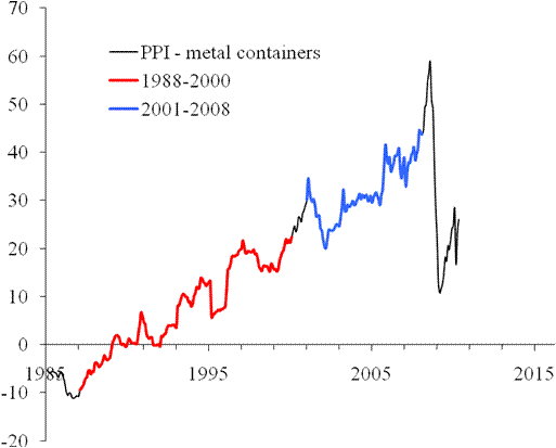
In this post, we revisit the trends in the PPI of three commodities related to metals: steel iron, nonferrous metals, and metal containers. Originally, these items were studied in our article [4]. This is a regular revision with the next scheduled to the end of 2010.

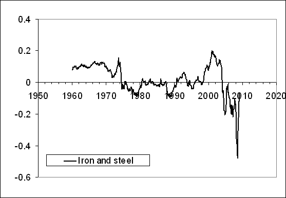
1. Figure 1 compares the original (upper panel), revised (middle panel) and the newly updated differences. According to [4]:
“the normalized difference between the PPI and the index for iron and steel (101) is characterized by the presence of a sharp decline between 2001 and 2008: from +0.2 to -0.4. Between 1980 and 2000, the curve fluctuates around the zero line, i.e. there was no linear trend in the absolute difference. One could expect the negative trend is now transforming into a positive one.“

A year ago we wrote:
“Between March and June 2009, the difference continued to increase, and likely reached its peak in June (Figure 2). In July or August 2009, the difference will stall around its peak value and then will start to decrease. As a result, the index for iron and steel will be growing faster than the PPI. In the short run, one can expect a fast recovery of iron and steel prices to the level observed in January-March 2008, i.e. the index will reach the level 210 to 220. However, this recovery will not stretch into 2011, and the index of iron and steel will be declining in the long run to the level of 2001, as depicted in Figure 3. In other words, the period between 2008 and 2010 is characterized by very high volatility, which will fade away after 2011. “

This prediction was right, as Figures 2 and 3 in this post demonstrate.

2. According to [4]:
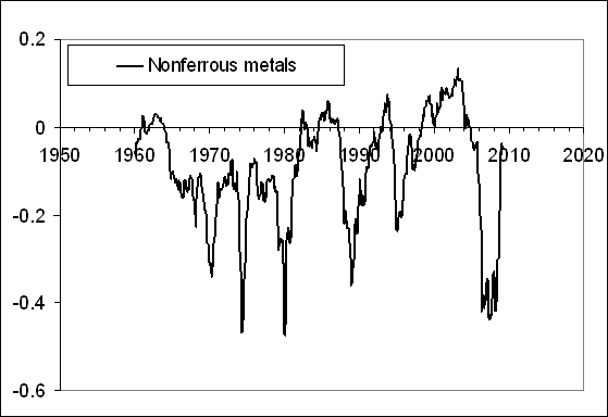
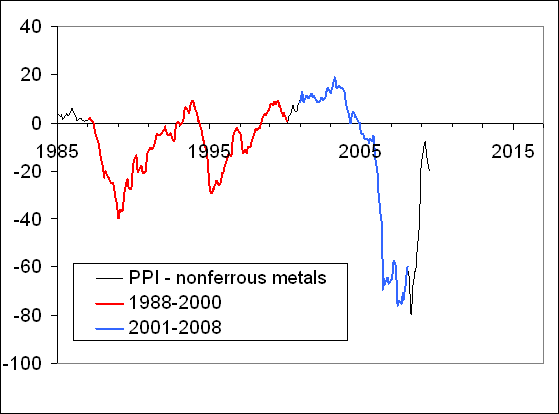
“the index for non-ferrous metals (102) shows an example of the absence of sustainable trends in the normalized difference. The curve is rather a comb with teeth of varying width. Although varying, the distance between consecutive troughs is several years at least. Therefore, one should not expect a quick recovery in the price for nonferrous metals”.

A year ago we wrote:
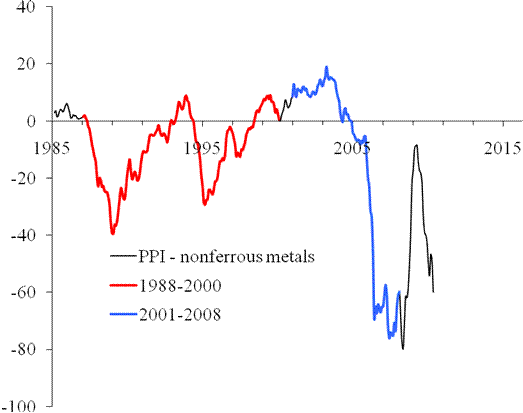
Figure 4 displays the original and updated predictions. There is almost nothing to add to the previous statement. The recovery in March-June 2009 is likely only a short-term one, as the past experience shows.

We also display in Figure 4 the newly updated trajectory. As forecasted, the producer price index of nonferrous metals has regained its price setting power, and the March-June 2009 excursion in the difference was only temporary. It should not last long, however.


3. It was stated in [4] that,
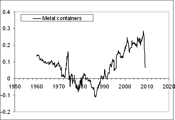
“the index for metal containers (103) provides an excellent example of linear trends in the normalized difference. There are two distinct periods between 1960 and 2008 with a turning point in 1987. A sudden drop in the difference in the end of 2008 may symbolize the start of transition to a new period with a negative trend. Then the price for metal containers will be increasing at an elevated rate, i.e. the index will get back its price setting power.”

A year ago we wrote:
Figure 5 presents the original and updated versions of the difference between the PPI and the index of metal containers. The negative overshoot in the difference reached its peak in March and currently the difference started to increase. One can not exclude short-period oscillations in the near future. The future of the index for metal containers is vague.

The difference was on an upward trend since June 2009 with a short-period fluctuation, as expected. The evolution along the positive trend should continue into 2011, i.e. the price index of metal containers will be losing its pricing power relative to the overall PPI.


Conclusion
Our simple predictions were good enough and validate the general concept of the sustainable trends in the CPI and PPI differences. Will keep reporting on the further developments.




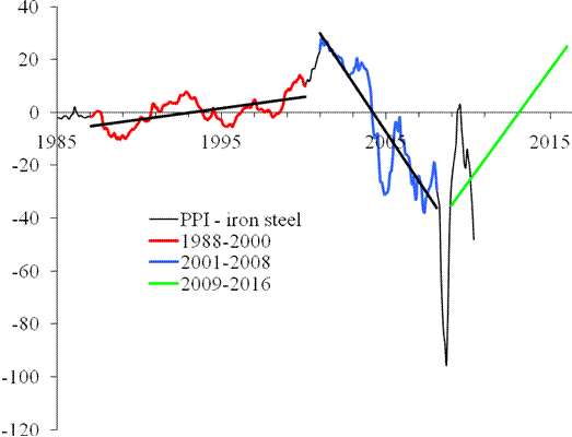
Figure 1. Upper panel: The evolution of the difference between the PPI and the price index of iron and steel between July 1985 and March 2009 (borrowed from [4]). Middle panel: Same for the period between 1985 and June 2009. Red and blue lines highlight segments between 1988 and 2001, and from 2001 to 2008, respectively. Green line predicts the evolution of the difference after 2008, as a mirror reflection of the linear trend between 2001 and 2008. Lower panel: The difference updated for the period between June 2009 and April 2010. As expected, the difference has been decreasing during the reported period and sank below the new trend (green). The trajectory has to turn up in the near future and reach the new trend by July 2011. This means that the price index for iron and steel will be growing at a lower rate than the overall PPI.



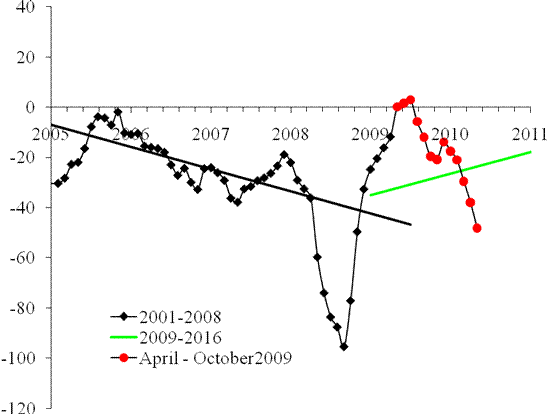
Figure 2. Upper panel: The evolution of the difference between the PPI and the price index of iron and steel between January 2005 and June 2009. Red line predicts the evolution of the difference after 2008. Red circles represent the difference between April and June 2009. We expect the difference will start growing in August-September 2009. Lower panel: The newly updated trajectory. The difference precisely obeyed our prediction a year ago and sank below the green line (new trend).



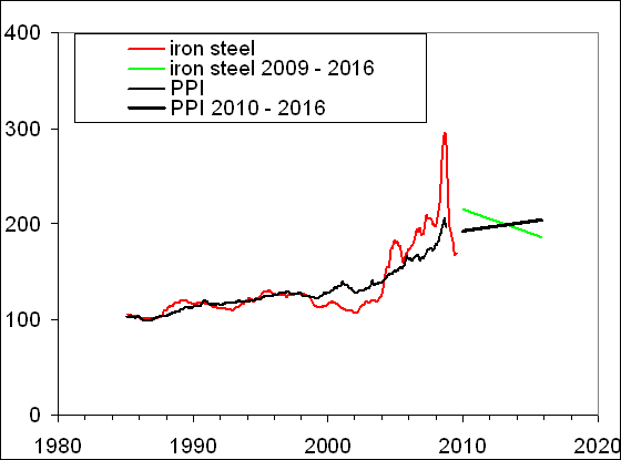
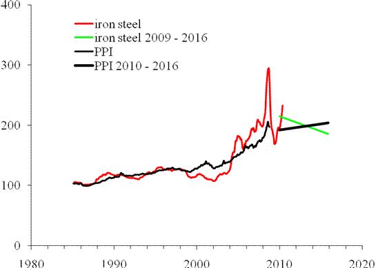
Figure 3. Upper panel: The evolution of the PPI, the index for iron and steel, and their difference in the long-run between 2009 and 2016. The index for iron and steel is predicted to decrease from the level of 220, which it will reach by the end of 2009, to ~185 in 2016. Accordingly, the difference will be growing as shown in Figure 1. The PPI will be also slowly growing. Lower panel: The newly updated trajectory.






Figure 4. Upper panel: The evolution of the difference between the PPI and the index of nonferrous metals from 1960 to March 2009 (borrowed from [4]). Middle panel: Same as in the upper panel for the period between 1985 and June 2009. There are no linear trends in the difference, but its behavior demonstrates a clear periodic structure with relatively deep but short troughs, which reflect the fast growth in the PPI for nonferrous metals. The last excursion ended in 2009. A period of hovering near the zero line is expected. Lower panel: The newly updated trajectory. As forecasted, the producer price index of nonferrous metals has regained its price setting power, and the March-June 2009 excursion in the difference was only temporary. It should not last long, however.




Figure 5. Upper panel: The evolution of the difference between the PPI and the index of metal containers from 1960 to March 2009 (borrowed from [4]). Middle panel: Same as in the upper panel for the period between 1985 and June 2009. There are distinct linear trends in the difference. One can not exclude that the fall in the difference is a start of the transition to a new trend. Lower panel: The newly updated trajectory.


References

1. Kitov, I., Kitov, O., (2008). Long-Term Linear Trends In Consumer Price Indices, Journal of Applied Economic Sciences, Spiru Haret University, Faculty of Financial Management and Accounting Craiova, vol. 3(2(4)_Summ), pp. 101-112.
2. Kitov, I., (2009). Apples and oranges: relative growth rate of consumer price indices, MPRA Paper 13587, University Library of Munich, Germany.
3. Kitov, I., Kitov, O., (2009). A fair price for motor fuel in the United States, MPRA Paper 15039, University Library of Munich, Germany,
4. Kitov, I., Kitov, O., (2009). Sustainable trends in producer price indices, Journal of Applied Research in Finance, v. 1, issue 1.
5. Kitov, I., Kitov, O., (2009). PPI of durable and nondurable goods: 1985-2016, MPRA Paper 15874, University Library of Munich, Germany
6. Kitov, I., (2009). Predicting gold ores price, MPRA Paper 15873, University Library of Munich, Germany
7. Kitov, I., (2009). Predicting the price index for jewelry and jewelry products: 2009-2016, MPRA Paper 15875, University Library of Munich, Germany
8. Kitov, I. (2010). Deterministic mechanics of pricing. LAP Academic Publishing, Saarbrucken, Germany.