Validation of the modified Okun's law for Germany

In the upper panel of  figure 1, we present the evolution of the cumulative inflation (the sum of annual inflation estimates) in Germany. There are two curves as defined by the CPI and dGDP between 1970 and 2018. Both variables are normalized to their respective values in 1970. Since 1996, the dGDP curve is above the CPI one and this configuration we interpret as economic super-performance. This effect is likely related to the EU financial rules with the ECB in Frankfurt. In the past, Germany has weaker performance and the EU leadership made it a super-economy. In the middle panel, the inflation rates are shown for both variables. In the lower panel, we present the difference between the CPI and dGDP curves in the upper and middle panels. One can see that the difference between the cumulative curves has several quasi-linear segments. The change in the slope between these segments in most likely related to the multiple revision to the dGDP definition. We have already used this observation of the segmented character of the real GDP estimates in order to assess our Okun’s-law-like model of the link between the change in unemployment and the change in real GDP per capita. The years of breaks in the dGDP time series are not easy to estimate from the lower panel of Figure 1 and we allow the LSQR method to find these years when minimizing the RMS residuals.

  

Figure 1. Upper panel: The evolution of the cumulative inflation (the sum of annual inflation estimates) as defined by the CPI and dGDP between 1970 and 2018. Both variables are normalized to their respective values in 1970.  Middle panel: The dGDP and CPI inflation estimates. Lower panel: The difference between the CPI and dGDP curves in the upper and middle panels.    

 

As for other countries, we minimize the model residuals, i.e. determine the break years together with the regression coefficients. For Germany, the best fit model between 1971 and 2018 is as follows:

           du_p = -0.42dlnG + 1.50, 1970>t≥1984

du_p = -0.555dlnG + 0.700,  1985≥t≥1992

du_p = -0.450dlnG + 1.300,  1993≥t≥2006

du_p = -0.450dlnG + 0.400,            t≥2007     (1)

where du_p – one-year change in the (OECD) the unemployment rate, G – real GDP per capita (2011 prices). The break years are determined automatically. Figure 2 presents the measured and predicted rate of unemployment (upper panel), the model residual error (middle panel), and the regression of the measured and predicted time series. The overall fit (Rsq.=0.88) is more when excellent with the break years close to those expected from Figure 1. One of the largest model errors in the residual time series was observed in 1990. This is most likely related to the reunification and merging of two time series belonging to different economies. When this spike is excluded, the standard deviation falls from 0.99% to 0.76%, and Rsq increases from 0.88 to 0.92. 

 The modified Okun’s law linking the change in the unemployment rate and the change in the real GDP per capita is validated by new data for Germany for the period between 2010 and 2019.

  

Figure 2. Upper panel: The measured rate of unemployment in Germany between 1970 and 2018, and the rate predicted by model (1) with the real GDP per capita and the unemployment rate published by the MPD. Middle panel: The model residual: stdev=0.99%. When the 1991 reading is excluded, stdev=0.76%.  Lower panel: Linear regression of the measured and predicted time series. Rsq. = 0.88.  

 

Modern professional sport is an ultimate expression of gender and race segregation

I had a post on the Winter Olympics as an example of hostile racial segregation. The winners of the Olympics have the same fame and honor as the winners of the (summer) Olympic Games. They almost all belong to one race and this predominance cannot be resolved - no natural snow and ice for the majority of UN countries. This segregation is based on historical prejudice.  It is even more outrageous because modern sport is professional and the absence of equal conditions is the worst expression of all kinds of inequality, including economic. 

Another example of professional segregation is the gender split in all major competitions. I have passed a few programs and exams on gender equality which definitely proved that the professional quality of males and females as well as of people of all races and sexual orientations is at least equal. As mentioned above - modern sport is a paid professional activity and thus there should be no gender/race segregation in sport. I have written a few papers on gender and racial income inequality in the USA and UK (e.g. 1, 2, 3)  which has to eliminated by all means. Income inequality in sports is based on one principle - competitions are split into two gender groups. 

Our duty is to fight against gender and racial segregation in sport. All sportspersons have a natural right to compete in equal conditions - no gender segregation. 

The modified Okun's law for France. Model validation with Rsq=0.98

 In the upper panel of Figure 1, we present the evolution of the cumulative inflation (the sum of annual inflation estimates) in France. There are two curves as defined by the CPI and dGDP between 1955 and 2018. Both variables are normalized to their respective values in 1955. Since 1985, the dGDP curve is above the CPI one and this configuration we interpret as economic underperformance. Also, we reported in this post that France has very low annual increment of the real GDP per capita. This effect is likely related to the EU financial rules. In the past, France and other European countries with underperforming economics forced price inflation in order to make exports more attractive due to lowering the exchange rate. In the middle panel, the inflation rates are shown for both variables. In the lower panel, we present the difference between the CPI and dGDP curves in the upper and middle panels. One can see that the difference between the cumulative curves has several quasi-linear segments. The change in the slope between these segments in most likely related to the multiple revision to the dGDP definition (e.g., imputed rent). We have already used this observation of the segmented character of the real GDP estimates in order to assess our Okun’s-law-like model of the link between the change in unemployment and the change in real GDP per capita. The years of breaks in the dGDP time series are not easy to estimate from the lower panel of Figure 1 and we allow the LSQR method to find these years when minimizing the RMS residuals.           

Figure 1. Upper panel: The evolution of the cumulative inflation (the sum of annual inflation estimates) as defined by the CPI and dGDP between 1955 and 2018. Both variables are normalized to their respective values in 1961.  Middle panel: The dGDP and CPI inflation estimates. Lower panel: The difference between the CPI and dGDP curves in the upper and middle panels.    

As in the previous posts, we minimize the model residuals, i.e. determine the break years together with the regression coefficients. For France, the best fit model between 1962 and 2018 is as follows: 

du_p = -0.134dlnG + 0.750, 1962>t≥1984

du_p = -0.255dlnG + 0.620,  1985≥t≥1999     

du_p = -0.520dlnG + 0.355,            t≥2000     (1) 

where du_p – one-year change in the (OECD) the unemployment rate, G – real GDP per capita (2011 prices). The break years are determined automatically. Figure 2 presents the measured and predicted rate of unemployment (upper panel), the model residual error (middle panel), and the regression of the measured and predicted time series. The overall fit (Rsq.=0.98) is more when excellent with the break years close to those expected from Figure 1. One of the possible reasons is that France has a good set of methods and procedures to measure/estimate economic parameters. This approach does not avoid data incompatibility problems, however, and statistical analysis needs extra efforts to distinguish between actual economic structural breaks and ignorance of basic procedures. The importance of data quality is best illustrated by an example in Figures 3 and 4, where two GDP per capita estimates from the OECD and MPD are compared. One can see that these two agencies provide quite different estimates. The use of the MPD estimates would change the statistical model. We do not know whose estimates are more accurate, but the OECD time series gives excellent results.

  

Figure 2. Upper panel: The measured rate of unemployment in France between 1960 and 2018, and the rate predicted by model (1) with the real GDP per capita and the unemployment rate published by the OECD. Middle panel: The model residual: stdev=0.50%. Lower panel: Linear regression of the measured and predicted time series. Rsq. = 0.98. 

Figure 3. Comparison of the real GDP per capita estimates reported by the OECD and Maddison Project Database. Both time series are normalized to their respective levels in 1960. 

Figure 4. The ratio of the OECD and MPD real GDP per capita estimates between 1960 and 2018.

The modified Okun's law for Canada. Model validation

 In our previous post, we revisited and validated our version of Okun’s law for the USA with new GDP and unemployment data for the years between 2010 and 2019. The revised model accurately describes the new data and three quarters of 2020, i.e. the original model is validated. In order to reach the best fit between the measured and predicted unemployment rates, we introduced a structural break in 2010 as related to the change in real GDP definition. 

In this post, we apply the same approach to Canada and start with the CPI and GDP deflator difference, which is used to reveal definitional breaks in the dGDP estimates. Obviously, such breaks in the dGDP creates breaks in the real GDP per capita estimates, and thus, in the statistical estimates associated with our model. One needs to find such breaks and allow the model to compensate for corresponding disturbances. At this stage, we ignore well-known steps in the unemployment rate estimates (see, TP-66 – CPS Design and Technology) related to the change in the population controls after the decennial censuses, e.g. the 2010 census. Such steps could be accurately compensated by dummy variables. More efforts are needed to investigate this problem and find the years when such steps were introduced in the labor force statistics.

 In the upper panel of Figure 1, we present the evolution of the cumulative inflation (the sum of annual inflation estimates) as defined by the CPI and dGDP between 1962 (we use the OECD data for the unemployment rate since 1961) and 2018. Both variables are normalized to their respective values in 1961. From the very beginning, the dGDP curve is above the CPI one and this configuration we interpret as economic underperformance. Another indicator of underperformance is the average annual increment of the real GDP per capita (from the Maddison Project Database) of $533 (2011 prices) compared to $643 in the USA – the biggest trade partner. In the middle panel, the inflation rates are shown for both variables. In the lower panel, we present the fit between the CPI and the dGDP cumulative inflation curves after correction of the latter in 1962 (coefficient 0.8), 1977 (0.8*1.4=1.12) and 2003(0.8*1.4*0.77=0.86). There was a period between 1977 and 2003 when the CPI grew faster than the dGDP.

  

Figure 1. Upper panel: The evolution of the cumulative inflation (the sum of annual inflation estimates) as defined by the CPI and dGDP between 1961 and 2018. Both variables are normalized to their respective values in 1961.  Middle panel: The dGDP and CPI inflation estimates. Lower panel: The fit between the CPI and the dGDP cumulative inflation curves after correction of the latter in 1962, 1977 and, 2003 (see text).   

 

In our model, we are looking for breaks near the years and obtain the following intervals and coefficients: 

du_p = -0.270dlnG + 1.130, 1977>t≥1970

du_p = -0.281dlnG + 0.303,  2000≥t≥1978     

du_p = -0.280dlnG + 0.505,  2009≥t≥2001              

du_p = -0.350dlnG + 0.180,           t≥2010     (1)

 

where du_p – one-year change in the (OECD) unemployment rate, G – real GDP per capita (2011 prices). The break years are slightly different from those estimated from the inflation curves in Figure 1. This is likely due to the higher sensitivity of the predicted unemployment rate to the coefficients in (1). The cumulative inflation curves in the upper panel of Figure 1 are both synchronously corrected in many revisions through their whole length. The estimates of the unemployment rate are obtained in the Current Population Surveys and represent independent estimates. The unemployment values are also corrected in the revisions to unemployment definition and when new population controls estimated after the decennial censuses. The original estimates cannot be changed but rather synchronously corrected. The rate of unemployment is an independent economic variable consisting of independent measurements. The predicted rate of unemployment depends on the integral value of the real GDP per capita. This makes the predicted value to be very sensitive to the GDPpc evolution. In other words, the current prediction, u_p, depends on the initial value, u(t₀), and the whole path of the GDPpc between t₀ and the current time. This is 49 years for Canada and 68 for the USA. The new readings of the unemployment rate and GDPpc (2011 to 2019) validate the model, which links the change in the rate of unemployment and the relative growth rate of the real GDP per capita in Canada.

 

Figure 2. Upper panel: The measured rate of unemployment in Canada between 1970 and 2019, and the rate predicted by model (1) with the real GDP per capita published by the MPD and the unemployment rate reported by the OECD. Middle panel: The model residual: stdev=0.62%. Lower panel: Linear regression of the measured and predicted time series. Rsq. = 0.87. 

 

 

We have validated our model allowing for an accurate prediction of GDP growth using unemployment estimates

 According to the gap version of Okun’s law, there exists a negative relation between the output gap, (Y^p-Y)/Y^p, where Y^p is potential output at full employment and Y is actual output, and the deviation of the actual unemployment rate, u, from its natural rate, uⁿ. The overall GDP or output includes the change in population as an extensive component which is not necessary dependent on other macroeconomic variables. Econometrically, it is mandatory to use macroeconomic variables of the same origin and dimension. Therefore, we use real GDP per capita, G, and rewrite Okun’s law in the following form: 

            du = a + bdlnG                                   (1) 

where du is the change in the rate of unemployment per unit time (say, 1 year); dlnG=dG/G is the relative change rate in real GDP per capita, a and b are empirical coefficients.  Okun’s law implies b<0.

The intuition behind Okun’s law is very simple.  Everybody may feel that the rate of unemployment is likely to rise when real economic growth is very low or negative. An economy needs fewer employees to produce the same or smaller real GDP also because of labor productivity growth.

When integrated between t₀ and t, equation (1) can be rewritten in the following form: 

u_t = u₀ + bln[G_t/G₀] + a(t-t₀)  + c          (2) 

where u_t is the rate of unemployment at time t. The intercept c≡0, as is clear for t=t₀.  Instead of using the continuous form (2), we calculate a cumulative sum of the annual estimates of dlnG with appropriate initial conditions. By definition, the cumulative sum of the observed du’s is the time series of the unemployment rate, u_t. Statistically, the use of levels, i.e. u and G, instead of their differentials are superior due to suppression of uncorrelated measurement errors.  

We showed (Kitov, 2011) the necessity of structural breaks in (1). Therefore, we introduced floating structural breaks in (2), which years have to be determined by the best fit. Thus, relationship (2) should be split into N segments. The integral form of Okun’s law should be also split into N time segments:

 u_t = u₀    + b₁ln[G_t/G₀]       + a₁(t-t₀),    t<t_s1                                                                                      

u_t = u_s1   + b₂ln[G_t/G_ts1]    + a₂(t-t_s1),    t_s2≥t ≥t_s1…

u_t = u_sN-1 + b_Nln[G_t/G_tsN-1] + a_N(t-t_sN-1), t_sN≥t ≥t_sN-1              (3) 

In 2011, we started with the U.S. The LSQR method applied to the integral form of Okun’s law (3) results in the following relationship:           

du_p = -0.406dlnG + 1.113, 1979>t≥1951

du_p = -0.465dlnG + 0.866, 2010≥t≥1979                (4) 

where du_p is the predicted annual increment in the rate of unemployment, dlnG is the relative change rate in real GDP per capita per year. A structural break around 1979 was found. It divides the whole 60-year interval into two practically equal segments. Figure 1 displays the measured and predicted rate of unemployment in the U.S. since 1951. The agreement between these curves is excellent with a standard error of 0.55%. The average rate of unemployment for the same period is 5.75% with a mean annual increment of 1.1%.  This is a very accurate model of unemployment with R²=0.89. Hence, our model (the integral Okun’s law) explains 89% of the variability in the rate of unemployment between 1951 and 2010 with the model residual most likely related to measurement errors.  Statistically, there is not much room for any other variables to influence the rate of unemployment, except they are affecting the real GDP per capita. 

Figure 1.  The observed and predicted rate of unemployment in the USA between 1951 and 2010. 

Our initial model worked well and its performance can be further validated by new data. Almost ten years passed and now we have two excellent opportunities to check the model: new readings for the previous years since 2010 and the extremely deep fall in the real GDP per capita accompanied by the unprecedented growth in the rate of unemployment in the USA, both induced by the COVID-19 pandemic. The latter is a dynamic effect of an exogenous and non-economic force. This is the best test of the link between the real GDP per capita and the unemployment rate. 

In our previous post, we supposed that the years between 2010 and 2019 have to be used to estimate the regression coefficient after the 2010 break. This structural break is related to the change in real GDP definition as one can see in Figure 2 from our previous post. In the upper panel of Figure 2 we present the evolution of the cumulative inflation (the sum of annual inflation rates) as defined by the CPI and dGDP between 1971 and 2020. Both variables are normalized to their respective values in 1970.  In the middle panel, the dGDP cumulative inflation is multiplied by a factor of 1.26 after 1979. The deviation since 1979 might be induced by a break in the GDP time series according to the comprehensive NIPA revision. After 2010, the CPI and dGDP curves still deviate, however. This effect is observed in new data and is likely associated with another break in the GDP time series. In the lower panel, we use a new coefficient of 0.8 in order to fit the CPI and dGDP after 2010. The overall fit is good and the total factor for this period is 0.8*1.26=1.00. It seems the old GDP definition is used after 2010.  

Figure 2. Upper panel: The evolution of the cumulative inflation (the sum of annual inflation rates) as defined by the CPI and dGDP between 1971 and 2020. Both variables are normalized to their respective values in 1970.  Middle panel: The dGDP cumulative inflation is multiplied by a factor of 1.26 after 1979. This deviation is induced by a break in the GDP time series according to the comprehensive NIPA revision). After 2010, the CPI and dGDP curves still deviate. This effect is observed in new data and is likely associated with another break in GDP time series. Lower panel: A new coefficient of 0.8 is used to fit the CPI and dGDP after 2010. The fit is good and the total factor for this period is 0.8*1.26=1.00. It seems the old GDP definition is used after 2010.   

The main result of our meticulous inspection of the CPI and dGDP deviation is the presence of breaks in data (i.e. data is not compatible in time) due to major revisions to the real GDP definition. Such a break was used in our version of Okun’s law for the USA as described by equation (4). The 2010 break may extend equation (3) to three different segments: 1951 to 1979, 1980 to 2010, and after 2010, with three different sets of coefficients. When the 1979-to-2010 set of coefficients is applied to the data after 2010 one obtains the curve shown in Figure 3, which does not match the measured rate of unemployment. Therefore, we apply the standard LSQR procedure to estimate a new set of coefficients for the period after 2010. The preliminary analysis gives the following model:           

du_p = -0.406dlnG + 1.122, 1979>t≥1951

du_p = -0.465dlnG + 0.899, 2010≥t≥1979       

du_p = -0.260dlnG  - 0.250,           t≥2010                 (5) 

Figure 4 illustrates the model predictive power. In the upper panel, the measured rate of unemployment in the USA between 1951 and 2019 is compared with the rate predicted by model (5) with the real GDP per capita published by the BEA. The rate of unemployment is borrowed from the BLS. In the middle panel, the model residual errors are presented with a standard deviation of 0.49% and the mean unemployment rate of 5.8%. The lower panel depicts the linear regression of the measured and predicted time series with Rsq.=0.89. Hence, the new set of coefficients provides an excellent match between the measured and predicted values, i.e. the model linking the change in the unemployment rate and the change in real GDP per capita is validated by the data between 2010 and 2019.

Figure 3. When the 1979-to-2010 set of coefficients is applied to the data after 2010 the predicted curve does not match the measured one.

Figure 4. Upper panel: The measured rate of unemployment in the USA between 1951 and 2019 and the rate predicted by model (5) with the real GDP per capita published by the BEA. Middle panel: The model residual. Lower panel: linear regression of the measured and predicted time series. Rsq = 0.89.  

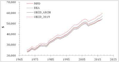
The ultimate validation test would be the model prediction for 2020, when the rate of unemployment changes by 10%  per quarter and the real GDP per capita falls by 35% in one quarter and then jumps back by 30%. It will be our next step after we present the prediction obtained using the MPD estimates of the real GDP per capita. Figure 5 shows that the MPD gives a slightly better fit with Rsq=0.91. This is just marginal improvement but it is important in terms of the methodology of statistical estimates with not perfect data measurements.  Finally, Figure 6 presents the rate of unemployment predicted for the three quarters of 2020. The spike in the second quarter is extremely accurately predicted with the model (5) estimated for the period between 2010 and in 2019. It is a good indicator that the model is still applicable and there were no NIPA revisions. 

Interestingly, the third quarter demonstrates a large prediction error – 5.3% instead of the measured value of 8.8%. The predicted unemployment rate is obtained with the real GDPpc growth of 30% in the third quarter.  The first GDP estimates for the third quarter might be highly overestimated. If the measured value of 8.8% is correct, the GDPpc growth has to be only 17% from the previous quarter.  We will follow the BEA releases with updated GDP estimates as well as the BLS releases with new estimates of the unemployment rate. The fourth quarter and the whole of 2020 is the next challenge for our Okun’s law version. 

In any case, one can use the unemployment estimates for an accurate prediction of the GDP growth!

 

Figure 5. Same as in Figure 4 with the MPD estimates of the real GDPpc.  

 

Figure 6. The rate of unemployment predicted for three quarters of 2020. The spike in the second quarter is extremely accurately predicted with the model (5) for the period after 2010. The third quarter demonstrates a large discrepancy, but the first GDP estimates might be highly inaccurate.   

Time to validate economic models: data quality analysis for the relationship between unemployment and real GDP

 The driving forces behind the change in unemployment (rate) in developed economies represent a very important and actual problem for the modern economic theory. For example, there exists an opinion that the change in unemployment may manifest tangible structural changes in the labor market. The COVID-19 pandemic is a natural non-economic (exogenous forces) experiment to test and validate all economic theories of unemployment. One can expect major changes in the overall organization of all economies (developed, emerging, etc.) when significant parts of them are suppressed or just decimated due to non-economic reasons. In this blog, we addressed the problem of structural unemployment by modeling the rate of unemployment with Okun’s law, i.e. the relationship of unemployment and real GDP growth. 

The COVID-19 pandemic is a deciding/survival opportunity for any quantitative economic theory like Okun’s law. Obviously, all descriptive economic theories never take data seriously, and these religious sects have their own apologists and believers: “In the beginning was the Word”.  In a series of future posts, we are going to revisit and validate our previous results obtained for a specific version of Okun’s law developed in a series of papers. The last overview of our empirically estimated Okun-style models for selected developed countries (the United States, France, the United Kingdom, Australia, Canada, and Spain) was published in 2011. The quantitative results suggest the absence of structural unemployment in the studied developed countries. The persistence of high unemployment is completely related to a low rate of real economic growth. 

This overview used the data between 1950 and 2009 from two principal sources – the Total Economy Database of the Conference Board and the OECD. Currently, the data on real GDP per capita and unemployment are available for the years between 2010 and 2019. We use the same data sources (Maddison Project Database instead of the TED) and compare the selected time series with similar time series from the BEA and BLS. 

In our previous work, we had to introduce (virtual) structural breaks in Okun’s law in order to improve the agreement between the change in the unemployment rate and real GDP per capita. As we described in several posts in December 2020, such breaks likely manifest artificial changes in definitions of unemployment and real GDP rather than actual shifts in the economic behavior of the variables in Okun’s law. The crucial importance of data quality and consistency for quantitative analysis makes is mandatory to check all time series of unemployment, employment, labor force, and real GDP per capita for definitional breaks and also to compare similar time series from different sources. Any deviation between similar time series from different sources should be considered as an estimate of measurement accuracy and resolution.  

To begin with, we compare the CPI and GDP deflator (dGDP) in the USA since 1929. The deviation between these two price inflation estimates as discussed in details (post2011, post2020) and here we would like to highlight the change in coefficients needed to match the CPI and dGDP curves. Also, we include the Personal Consumer Expenditure (PCE) index in the discussion. The PCE is a major component of the Gross Domestic Product. Figure 1 presents all three indices in panel a), where the corresponding time series are normalized to their respective values in 1929, i.e. 1929 is the reference year. The (total price increase) CPI curve starts to deviate from the PCE and dGDP curves since the late 1970s.  The PCE and dGDP curves are very close in their cumulative representation. Panel b) in Figure 1, depicts the cumulative inflation, i.e. the sum of annual inflation rates, for the three indices. This representation is more sensitive to the differences in the indices and one can observe slight deviations between the PCE and dGDP, as well as the discrepancy between the PCE and dGDP in the late 1940s.

 a) 

b)

Figure 1. a) The price increase as described by the CPI, PCE, and GDP deflator in the USA since 1929. All curves are reduced to their respective levels in 1929. Data are borrowed from the BEA and BLS. The CPI price increase becomes higher than the PCE and GDP price growth since 1979. b): The cumulative inflation (i.e. the sum on annual inflation readings in percentage points) according to price indices: CPI, PCE, and GDP deflator. Deviations between the three curves are better seen in this representation.

 

Figure 2 depicts the differences between the annual inflation estimates and the cumulative inflation curves for all three pairs of the studied indices. Panel a) shows the CPI and dGDP differences. The difference between the cumulative inflation curves reveals the deviation between these two approaches to price inflation.  Before 1978, the difference between the CPI and dGDP curves was hovering in the range between -5 and +5. It looks like that the CPI was the basis of the GDP deflator. The period between 1981 and 2001 could be well approximated by a linear function. The years between 1978 and 1980 are like a spike or a correction distributed over 3 years. As we know, there was a comprehensive NIPA (national income and product accounts) revision around 1980 and the effect of this revision was distributed over years. It is not excluded that the comprehensive NIPA revisions may include new elements making the real GDP time series incompatible in time. 

Since we were limited to 2009 in our previous study in 2011, the segment between 2010 and 2019 is of the largest interest for the model validation. It is important to stress that there was a comprehensive NIPA revision in 2010. For Okun’s law, these revisions mean the change in the coefficients of linear regression between the GDP per capita and the rate of unemployment, i.e. virtual breaks in the dependence one can confuse with structural breaks in economic behavior. One can also pretend that the years between 2001 revision and 2010 revision to the GDP definition are characterized by a slightly lower slope of the different line than the years between 1982 and 2000. Potentially, there should be a break in 2001, but it might be too small to affect statistical estimates of our model. 

Panel b) in Figure 2 presents the same curves for the CPI-PCE pair. The PCE is close to the dGDP and the general features of the difference between cumulative inflation curves are similar to those in panel a). In panel c), the differences for the dGDP-PCE pair are presented. One can see that the dGDP and PCE indexes are slightly different. Interestingly, the level of variation in the differences between the CPI and PCE cumulative curves is higher before 1990 than after 1990. This observation is likely related to the improvement in the definition. 

a) 

b)

c)

Figure 2. a) The difference of the annual and cumulative inflation estimates for the CPI and  GDP deflator in the USA since 1929. b): The difference of the annual and cumulative inflation estimates for the CPI and the PCE in the USA since 1929.

 Figure 3 demonstrates that the PCE gives from 59% to 68% of the real GDP. Panel c) in Figure 3 is likely the most important for the success of the current study - it shows the change in various real GDP components in 2020. The quarter-to-quarter change rate in real GDP in the second quarter of 2020 was -36% and +30% in the third quarter.  The PCE dropped by 38.0% in the second quarter and increase by 36% in the third. 

According to our version of Okun’s law, the fall in real GDP per capita results in an increase in the rate of unemployment. The linear regression coefficient for the period before 2010 was -0.465 and the constant term was 0.9. When applied to the fall in the real GDP per capita these coefficients would give 21% unemployment rate in the second quarter. (Here we have to use the real GDPpc instead of real GDP.) The observed rate was 13.3%. The discrepancy is probably due to the break in the regression coefficients in 2010. To match the unemployment rate observed in the second quarter of 2020, the model needs the regression coefficient has to be ~0.25. The years between 2010 and 2019 have to be used to estimate the regression coefficient after the 2010 break. The recovery in the third quarter is also an important observation for the model validation. 

a) 

b)

c)

Figure 3. a) Components of the GDP. Personal Consumer Expenditures (PCE) varies between 59% and 68%. b) Contributions to Percent Change in Real Gross Domestic Product. c) The quarterly rate of change in real GDP components. 

In Figure 4, the GDP deflator is split into its major components and the total price change (panel a) and inflation rates (panel b) are presented. In panel c) we show the quarterly (y/y) estimates of the price inflation rates.  In 2020, only exports and imports demonstrate a negative inflation rate. The dGDP and PCE inflation rates are positive (0.6%). We are going to use the dGDP and PCE price inflation estimates in the extended model linking inflation, unemployment, and labor force. The accuracy of inflation estimates is crucial for this model.

a)

b) 

c)

Figure 4. a) The evolution of the GDP price deflator and its components since 1929. The GDP deflator is very close to the PCE, as the largest input to the GDP. b) Price inflation of the components in panel a). The largest inflation is related to Imports. c) Quarterly (y/y) inflation estimates for the GDP major components. Imports and exports demonstrate the largest fall in 2020. 

Finally, the real GDP per capita estimates may differ between the major providers of economic data. Figure 5 presents four different real GDP per capita curves for the USA: the Maddison Project Database, Bureau of Economic Analysis, and two curves from the OECD. Because of varying reference years and corresponding reference real GDPpc levels, the curves are similar is shape but have different levels. In the lower panel of Figure 5, the change rates (y/y) are presented and the difference between them is most prominent after 2010. The period between 2010 and 2020 is characterized by the highest uncertainty in GDP per capita. 

Figure 6 depicts the ratio of the MPD GDP per capita and three other time series, all 4 series are first normalized to their respective levels in 1970 and the ratios are calculated. As a result, all ratios start from 1 and one can see the discrepancy of the real GDP per capita estimates. For example, the MPD/BEA curve drops to 0.98 in 2015, and the other two ratios fall even deeper to 0.975. In standard statistical analysis, the results may differ, especially after 2010. Figure 7 illustrates the change in the real GDPpc estimates published by the same agency - OECD. One cannot exclude the possibility that the current estimates of any economic parameters are subject to revisions in the future, and these revisions may change statistical estimates for all economic relationships.  

Figure 5. Upper panel: Four real GDP per capita curves reported by different economic agencies. Lower panel: the reported change rates are slightly different between the agencies. 

Figure 6. The ratio of the MPD GDP per capita and three other time series.

Figure 7. The change in the real GDPpc estimates published by the OECD: OECD_ARCH – archived time series, OECD-2019 the most recent revision.