Paul Krugman compares inflation in US and Japan

Paul Krugman, after this piece admitting the general failure of economics, explains in here why inflation in Japan is very low (due to deflation expectations) and why the US will repeat all the way down. Except the future of the US inflation, i.e. deflation starting in  2012, there is no right explanation os the driving force behind price inflation. We explained the case of Japan five years ago, and predicted an extended period of deflation in the US six years ago. 

The performance of 10-year T-notes during deflation

In our previous article we presented a prediction of an extended period of price deflation in the U.S. since 2012. Our projection was made in 2006 and covers the period between 2006 and 2016. At least five years are characterized by negative inflation. The underlying model can also foresee beyond 2016 when some updated labour force projections are used (see Appendix). There is no expectation of a positive inflation rate at least in the 2010s. Deflation is a major risk for the U.S. economy and stock market. Therefore, one can consider a safer investment in Treasuries. Let us check various options. 

Currently (August 18, 2:15), T-notes and T-bonds have very low yields between 0.19% for 2-year T-notes and 3.55% for 30-year T-bonds. Since the predicted deflationary period will last at least 8-years one can choose between 7-year and 10-year T-notes. The former has the yield of 1.45% and the latter 2.15% (coupon 2.125%). Taking into account the predicted rate of inflation below -0.5% per year in the near future, one can evaluate the real yield as 3% in the next few years. This is a safe and relatively profitable investment during the poor years to come. The stock market will likely be stangnant if not  decaying.

 Appendix

The BLS has projected the level of labour force to increase from 154.300.00 in 2008 to 167.000.00 in 2018, i.e. by 0.8% per year on average. Considering the current fall in the rate of participation down to 64.5% (instead of 66%) which was expected only in 2018, we should decrease the projected level in 2018 by approximately 1.2%, i.e. to 165.000.000. Then, the rate of labour force growth is 0.66% on average between 2008 and 2018. According to our model the rate of consumer price inflation is driven by the change rate in labour force: 

CPI(t)=4.5dlnLF(t-3)/dt - 0.032 (1) 

where CPI(t) is the rate of consumer price inflation at time t, LF(t-3) is the level of labour force three years before the predicted rate of inflation. Using the average rate of labour force change between 2008 and 2018 one can estimate the average consumer price inflation between 2008 and 2018 as -0.3% per year. Since the years between 2008 and 2011 have a positive inflation rate the years after 2012 will have evens a smaller average inflation rate.  On average, I would estimate the future rate of inflation as -0.5% per year since 2012. However, during 2012 and 2013 it can be as low as -3%.  

Deflation is a long term threat for the stock market

Price deflation in the U.S. is an issue which attracts attention. For example, the FOMC statement implies very low inflation at a two year horizon. The two-year breakeven inflation rate is negative. As a result, economics blogs are also full of discussions around the near future of the overall price behaviour.  (Despite the explicit FOMC statement many experts expect a period of hyperinflation after two sessions of quantitative easing.) The danger of deflation has been demonstrated by Japan where the quantitative easing did not show any positive results.  

We predicted an extended deflationary period since 2012 five years ago. This prediction was based on a model describing inflation in developed countries as a linear and lagged function of labour force. In 2006, we published a forecast for the U.S. a ten year horizon using the following relationship:  

DGDP(t) = 4.0dlnLF(t-2)/dt – 0.03              (1)                       

 where DGDP is the GDP deflator at time t, and dlnLF(t-2)/dt  is the rate of growth in the level of labour force two years before, t-2. In equation (1), the slope is 4.0 and intercept is -0.03. Using (1) and various projections of labour force we estimated the rate of inflation between 2006 and 2016. Figure 1 compares the predicted rate of inflation with that observed between 2006 and 2010.  The agreement is very good considering the precision of inflation measurements and the labour force projection published by the CBO in 2004.  

For 2011, the model predicts the rate of inflation near 0.4%. The current fall in commodity prices and the deceleration in real economic growth both imply no price inflation in the second half of 2011. Hence, our prediction for 2011 from 2006 seems to be right.   

Between 2012 and 2016, the rate of inflation (as expressed by the GDP deflator) will be negative at the level between -0.5% and -1.2% (2013).  Obviously, the CBO labour force projection at a ten year horizon could not be too precise and actual values of the future inflation rate may differ from the predicted ones. However, the negative inflation trend is a serious and long term danger for the U.S. economy.

Figure 1. Predicted inflation rate for the period between 2006 and 2016 according to the CBO’s (2004) labour force projection.  A deflationary period starts in 2012.  

Deflation in consumer prices is also predicted by the current measurements of labour force. We estimated a similar relationship for the headline CPI. Five years ago the following relationship was obtained: 

CPI(t) = 4.5dlnLF(t-3)/dt – 0.032                (2) 

The time lag of three years (actually 2.5 years) provides the best fit between observed and predicted values.  In (2), the slope is larger than in (1). This difference expresses a larger volatility in consumer prices.  Figure 2 illustrates the agreement between the observed and predicted rate of consumer price inflation between 1960 and 2010.  At a three year horizon one can expect a significant fall in the rate of inflation, down to -4% per year.  This is a great threat for producers, consumers and the U.S. economy as a whole. 

The uncertainty in labour force measurements is directly mapped into high-amplitude fluctuations. These fluctuations represent banal measurement noise and can not be removed without improvements in the relevant BLS methodology and procedures. It is instructive that the largest fluctuations correspond to the years of decennial censuses. The Census Bureau has to smooth the difference between counted and projected population values (so called population controls) and the BLS ignores these steps. As usually, the most reliable readings correspond to the changes with the largest amplitude.

The best way to suppress this measurement noise is to use integral (cumulative) values.  Figure 3 displays the observed and predicted cumulative inflation curves starting from 1965. The predicted cumulative curve is obtained by a progressive summation of values from 1963 and is also shifted ahead by 2 years. There is an almost complete agreement between the cumulative curves for the whole period. The only small deviation occurred around 1993 and corresponds to a sharp drop of the rate of labour force growth as induced by the baseline working age population correction.

Figure 2. Measured inflation and that predicted from the dLF/LF (shifted 2 years ahead). An agreement is observed throughout the whole period with some short fluctuations in labour force potentially induced by the population corrections implemented by the Census Bureau in the census years. 

The predicted cumulative curve is very sensitive to free term in (2). Even the initial difference of 0.0001 results in a tangible deviation from the measured curve after 50 years. Therefore, the value of free term in (2) can be estimated with a good accuracy. It is important that the cumulative curves represent actually measured macroeconomic variables: labour force and price. Inflation and change rate are based on first differences of the original values and thus are much more sensitive to measurement errors.  

Figure 3. Comparison of the cumulative values of the observed and predicted inflation presented in Figure 2. The predicted curve starts from 1963 and is shifted by 2 years ahead. An agreement is observed with a notable change from convexity before 1980 to concavity one after 1980.

One can conclude that a deflationary period will likely start in 2012 and then may extend into the second half of the 2010s. Price deflation is a major risk for the stock market.  

Deflation in Japan. The other view

Our previous post showed that inflation in Japan can be completely explained by the change in labor force. Obviously, there are different (and wrong) explanations based on monetary policy of the Bank of Japan. Below is an abstract of  a working paper on this issue. In my view, it is absolutely worthless as not describing any period or major change in the inflation evolution. How can they seriously publish this kind nonsense?

Japan's Deflation and the Bank of Japan's Experience with Non-traditional Monetary Policy

This paper offers a brief summary of non-traditional monetary policy measures adopted by the Bank of Japan (BOJ) during the last two decades, especially the period between 1998-2006, when the so-called Zero Interest Rate Policy (ZIRP) and Quantitative Easing (QE) were put in place. The paper begins with a typology of policies usable at low interest and inflation rates. They are: strategy (i), management of expectations about future policy rates; strategy (ii), targeted asset purchases; and strategy (iii), QE. Alternatively, QE may be decomposed into a pure attempt to inflate the central bank balance sheet, QE0, purchases of assets in dysfunctional markets, QE1 and purchases of assets to generate portfolio rebalancing, QE2. Strategy (ii), when non-sterilized, is either QE1 or QE2. Using this typology, I review the measures adopted by the BOJ and discuss evidence on the effectiveness of the measures. The broad conclusion is that strategies (i) and (ii) have affected interest rates, while no clear evidence exists so far of the effectiveness of strategy (iii), or QE0. Strategy (ii) has been effective especially in containing risk/liquidity premiums in dysfunctional money markets; that is, QE1 has been effective. The effectiveness of QE2, however, is unclear. The strategies, however, have failed to bring the economy out of the deflation trap so far. I discuss some possible reasons for this and also implications for the current U.S. situation.

The GDP deflator in Japan

We have already mentioned that Japan is the best illustration of our concept linking inflation/unemployment to the change in labour force. In the previouspost on inflation in Japan, we modelled the overall CPI. Here we illustrate the long term equilibrium relation between the GDP deflator, DGDP, and labour force. All data were obtained from the OECD.

By trial-and-error, we seek for the best-fit coefficients in the linear and lagged link between inflation and labour force. Because of the structural (measurement related?) break in the 1980s, we have chosen the period after 1981 for linear regression, which is common for almost all economic studies related to Japan. By varying the lag and coefficients we have found the following relationship:

DGDP(t)= 1.9dLF(t-t₀)/LF(t-t₀) – 0.0084        (1)

where the time lag t₀=0 years; Figure 1 depicts this best-fit case. There is no time lag between the inflation series and the labour force change series in Japan. Free term in (1), defining the level of price inflation in the absence of labour force change, is close to zero but negative.

A more precise and reliable representation of the observed and predicted inflation consists in the comparison of cumulative curves shown in the lower panel of Figure 1. We always stress that the cumulative values of price inflation and the change in labour force are the levels of price and labour force, respectively. Therefore, the summation of the annual reading gives the original estimates of price and workforce, which when are converted into rates.

Another advantage of the cumulative curves is that all short-term oscillations and uncorrelated noise in data as induced by inaccurate measurements and the inevitable bias in all definitions are effectively smoothed out. Any actual deviation between these two cumulative curves persists in time if measured values are not matched by the defining relationship. The predicted cumulative values are very sensitive to free term in (1).

For Japan, the DGDP cumulative curves are characterized by very complex and unusual for economics shapes. There was a period of intensive inflation growth and a long deflationary period. The labour force change, defining the predicted inflation curve, follows all the turns in the measured cumulative inflation with the coefficient of determination R²=0.96. (Again, these are actually measured curves.) With shrinking population, and thus, labour force, the GDP deflator will be falling through 2050 and likely beyond.

Figure 1. Measured GDP deflator and that predicted from the change rate of labour force. Upper panel:  Annual curves smoothed with MA(3). Lower panel: Cumulative curves between 1981 and 2010. A good agreement between the cumulative curves illustrates the predictive power of our model.

Price deflation in Switzerland?

We have already presented several empirical quantitative models of price inflation in developed countries in this blog. Our major result is the existence of a long-term equilibrium link between price inflation and the rate of change of labour force. Statistically, these two macroeconomic variables are cointegrated in such countries as the USA, France, Canada, and Austria. In some countries, e.g. the UK and Japan, the length of reliable data is too short for cointegration tests to be significant. However, cumulative inflation is accurately predicted in all countries.

Switzerland is one of the most important (although a middle size one) world economies. The country's statistics is characterized by relatively lengthy observations of labour force (Figure 1) and inflation (Figure 2). Apparently, the labour force series has two breaks: one in 1974 of unknown nature and one in 1991, as the OECD (2008) informs:

Series breaks: From 1998, data are adjusted in line with the 2000 census. Prior to 1991, data refer only to persons who are gainfully employed at least six hours per week.

The link between inflation and labour force also has a break around 1987, as Figure 3 depicts. Same effect was observed in Austria, where the change in the link is completely explained be the introduction of the ILO definition of labor force and unemployment instead of national ones. Linear regression of the observed series on the predicted one is characterized by slope 0.74, free term 0.003, and R2=0.82. According to the well-know problem with OLS, the slope is underestimated. Otherwise, the agreement is excellent. We did not use the cumulative curves for the estimation of coefficients in the linear link between labor force and inflation for Switzerland since corresponding time series are not long enough to provide a robust estimate. Fortunately, the original inflation curve (CPI) oscillates with a significant amplitude, and one only needs to fit the peaks of the oscillations in order to find appropriate coefficients, as shown in the Figure.

Hence, we have price inflation defined by a linear function of labor force with both coefficients changing in 1987:

CPI(t)= 1.1*dLF(t-2)/LF(t-1) + 0.005, before 1987

CPI(t)= 2.0*dLF(t-2)/LF(t-1) + 0.055, after 1987

It is worth noting that the predicted curve has two segments and covers the period between 1967 and 2008. All in all, the predictive power of the model is good and timely fits major peaks and troughs. Because the lag between the change in labor force and inflation is two years one can foresee the change in prices at this time horizon. In Switzerland, one should not expect high price inflation since the level of labor force has not been growing fast enough during the last two decades. It is very likely that inflation will be very low or even negative (deflation) in Switzerland over the next decade due to demographic problems and ageing population.

Figure 1. The rate of labour force change in Switzerland according to national definition (NAC) and the definition adopted in the US.

Figure 2. Two definitions of the rate of price inflation in Switzerland: GDP deflator and CPI inflation according to OECD definition.

Figure 3. Upper panel: The rate of CPI inflation in Switzerland as predicted by the  model with a structural break neat 1987 related to the change in measuring units. Notice that the predicted series is smoothed with MA(3). Lower panel: Linear regression of the data in the upper panel.

On the likelihood of deflation in Canada

Three years ago we published a paper on inflation and unemployment in Canada, where we presented a model linking inflation and unemployment with the change in labor force. This earlier prediction was revisited in 2010 and demonstrated excellent predictive power of the original model. Today we add two more readings, for 2008 and 2009, to all time series and extend the prediction.

Skipping the part introducing data and presenting individual models linking inflation and unemployment to labor force separately, we revisit our generalized relationship. It gathers all individual ones. We find the best-fit coefficients for the generalized equation:

pi(t) = 3.8dLF(t-2)/LF(t-2) + 0.79UE(t-2) - 0.095 (1)

Figure 1 depicts the case associated with the data provided by the BLS. Both cumulative curves are very close. Moreover, these curves reveal three periods of different behaviour and prove that there was no change in the long-term equilibrium relation between these three studied variables.

The difference between the cumulative curves is very small compared to the net change between 1969 and 2004. Moreover, this difference decreases with time as Figure 2 shows. One can easily find that the coefficients obtained by linear regression of the CPI on the LF and UE do not provide such a closeness between cumulative curves as those coefficients, which are estimated by visual fit between the cumulative curves.

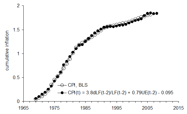
Figure 1. Comparison of cumulative curve for the measured CPI and that predicted using the BLS definition of labour force.

Figure 2. The difference between the cumulative curves in Figure 1.

Figure 3 demonstrates the advantages of the moving average technique applied to the annual measurements of labour force, unemployment, and CPI inflation in Canada. As discussed above, these measurements are characterized by random errors, which are weighted through years in accordance with benchmark measurements. It means that the average measurement error approaches zero for the increasing length of time series. Therefore, a five-year moving average, MA(5), should significantly suppress random errors and provide close cumulative curves, as one can observe in Figure 1.

Figure 3. Comparison of MA(5) curve for the measured CPI and that predicted according to relationship (1).

Considering the accuracy of the CPI prediction between 1971 and 2009, one can expect the rate of consumer price inflation in Canada to fall very close zero on average during the next 5 years. It is very likely that few years will bring negative inflation rates, i.e. formal deflation.

Bernanke and deflation

Deflation is the economic topic where the current  Chairman of the United States Federal Reserve Shalom Bernanke has got his nickname. We have been following the evolution of inflation in the USA for many years since predicted (2005)  that a deflationary period should start in 2012.  So, it is instructive to  compare the tools proposed by the Fed's chairman and actual situation. The most recent statement from the FRB on deflation was in the speech  on October 15.

... The significant moderation in price increases has been widespread across many categories of spending, as is evident from various measures that exclude the most extreme price movements in each period. For example, the so-called trimmed mean consumer price index (CPI) has risen by only 0.9 percent over the past 12 months, and a related measure, the median CPI, has increased by only 0.5 percent over the same period.2



... With long-run inflation expectations stable and with substantial resource slack continuing to restrain cost pressures, it seems likely that inflation trends will remain subdued for some time.

The longer-run inflation projections in the SEP indicate that FOMC participants generally judge the mandate-consistent inflation rate to be about 2 percent or a bit below. In contrast, as I noted earlier, recent readings on underlying inflation have been approximately 1 percent. Thus, in effect, inflation is running at rates that are too low relative to the levels that the Committee judges to be most consistent with the Federal Reserve's dual mandate in the longer run. In particular, at current rates of inflation, the constraint imposed by the zero lower bound on nominal interest rates is too tight (the short-term real interest rate is too high, given the state of the economy), and the risk of deflation is higher than desirable. Given that monetary policy works with a lag, the more relevant question is whether this situation is forecast to continue. In light of the recent decline in inflation, the degree of slack in the economy, and the relative stability of inflation expectations, it is reasonable to forecast that underlying inflation--setting aside the inevitable short-run volatility--will be less than the mandate-consistent inflation rate for some time. Of course, forecasts of inflation, as of other key economic variables, are uncertain and must be regularly updated with the arrival of new information.

and finally

Given the Committee's objectives, there would appear--all else being equal--to be a case for further action. However, as I indicated earlier, one of the implications of a low-inflation environment is that policy is more likely to be constrained by the fact that nominal interest rates cannot be reduced below zero. Indeed, the Federal Reserve reduced its target for the federal funds rate to a range of 0 to 25 basis points almost two years ago, in December 2008. Further policy accommodation is certainly possible even with the overnight interest rate at zero, but nonconventional policies have costs and limitations that must be taken into account in judging whether and how aggressively they should be used ...

So, the problem of approacing price deflation now is a big one. To implememnt a helicopter technology is not so easy.

On deflation, once again

Five years ago we developed an empirical model describing inflation in developed countries and published a forecast for the USA at a ten year horizon in 2006 (Kitov, 2006ab) as a linear and lagged function of labour force. For the USA the model is as follows:

DGDP(t) = 4.0dLF(t-2)/LF(t-2) – 0.03 (1)

where DGDP is the GDP deflator at time t, and LF is the level of labour force two years before, t-2. In equation (1), the slope of linear relationship is 4.0 and intercept is -0.03. With labour force constant (dLF=0), the overall price inflation in the USA would remain negative at the level of -3% per year. For inflation to be sustainable at the level of 2% (the fed’s unannounced target) the growth in labour force of 1.25% per year is required.

Eventually, the link between price inflation and labour force was successfully tested for cointegration (Kitov, Kitov, Dolinskaya, 2007) and validated using 1-D boundary elements methods (Kitov, Kitov, 2010). This links holds for other developed countries as well (Kitov, Kitov, 2010).

Figure 1 illustrates the linear and lagged relationship between inflation (GDP deflator) and the change rate of labour force in the USA for the period between 1960 and 2006. The estimates of the change rate of labour force are shifted by two years ahead in order to synchronize the predicted peaks of inflation with those actually observed in 1975 and 1984. Due to the uncertainty in the labour force (and inflation) measurements the most reliable readings correspond to the changes of the largest magnitude, as described by the BLS. Every sound model of price inflation must explain these peaks.

Figure 1. Measured inflation (GDP deflator) and that predicted from the dLF/LF (shifted 2 years ahead). An agreement is observed throughout the whole period with some short fluctuations in labour force potentially induced by the population corrections implemented by the Census Bureau in the census years.

Figure 2 presents two smoothed inflation curves – the measured and the predicted one. The smoothing was attained by a 7-year moving average, MA(7), with a one-year step. The predicted curve is shifted by 2.5 years (we used two time scales with a half-a-year shift) ahead in order to fit the inflation peak near 1978. The original (not shifted) predicted curve is also shown in order to illustrate that it is actually leading by 2.5 years.

Figure 2. MA(7) of the predicted and measured inflation. The prediction is made according to the relationship (1). The predicted curve is shifted by 2.5 years ahead.

Figure 3 displays the observed and predicted cumulative inflation curves starting from 1965. The predicted cumulative curve is obtained by a progressive summation of values from 1963 and is also shifted ahead by 2 years. There is an almost complete agreement between the cumulative curves for the whole period. The only small deviation occurred around 1993 and corresponds to a sharp drop of the rate of labour force growth as induced by the baseline working age population correction.

The predicted cumulative curve is very sensitive to free term in (1). Even the initial difference of 0.0001 results in a tangible deviation from the measured curve after 50 years. Therefore, the value of free term in (1) can be estimated with a good accuracy. With cumulative curves, one can obtain the most accurate coefficients solely on the basis of visual fit. Also, since these two cumulative curves have R2>0.999 and actually represent indexes one can replace the secular growth in the overall price as the cumulated growth in labour force two years before. In a sense, these curves are similar to conservation laws or integral equations in physics (Kitov, Kitov, 2010).

Figure 3. Comparison of the cumulative values of the observed and predicted inflation presented in Figure 1. The predicted curve starts from 1963 and is shifted by 2 years ahead. An agreement is observed with a notable change from convexity before 1980 to concavity one after 1980.

Relationship (1) can be used for a prediction at a larger time horizons using labour force projections made by various institutions. For example, the projections made by CBO (2004) and BLS (2005) undoubtedly indicate a decrease in the participation rate and a decaying growth rate of the working age population. According to these projections, staring from 2010, the annual increase in labour force will be less than 1,200,000 – the value separating inflation and deflation. Hence, the year of 2012 is likely to mark the beginning of the deflationary era in the USA (which hopefully is the global disaster the Mayans talked about) because of the two-year lag between the labour force change and inflation. Figure 4 details the prediction based on the CBO’s projection of the labour force. After peaked at 3.2% in 2007, the rate of price inflation has been at a gradual decrease, which will lead to the first red figure in 2012.

Hence, we are waiting an extended deflationary period in the USA since 2012.

Figure 4. Predicted inflation rate for the period between 2006 and 2016 according to the CBO’s (2004) labour force projection. A deflationary period starts in 2012.

References

Bureau of Labor Statistics. (2005a). Labor force projections to 2014: retiring boomers. Monthly Labor Review, November 2005.

Congressional Budget Office. (2004). CBO’s Projections of the labor force. September 2004.

Kitov, I. (2006a). Inflation, unemployment, labor force change in the USA, Working Papers 28, ECINEQ, Society for the Study of Economic Inequality,http://ideas.repec.org/p/inq/inqwps/ecineq2006-28.html

Kitov, I. (2006b). Exact prediction of inflation in the USA, MPRA Paper 2735, University Library of Munich, Germany

Kitov, I., Kitov, O., Dolinskaya, S. (2007). Inflation as a function of labor force change rate: cointegration test for the USA, MPRA Paper 2734, University Library of Munich, Germany

Kitov, I., Kitov, O. (2010). Dynamics of Unemployment and Inflation in Western Europe: Solution by the 1-D Boundary Elements Method, Journal of Applied Economic Sciences, Spiru Haret University, Faculty of Financial Management and Accounting Craiova, vol. V(2(12)_Summer), pp. 94-113.

Deflation is approaching US

At last, deflation is approaching the US. A new post by Mark Thoma @ Economist's View:


How close to deflation are we?



Interstingly, five years ago we calculated that a deflationary period should start in 2012 and publsihed this forecast in 2006: Exact prediction of inflation in the USA.



Below is Figure 9 from this paper. ALl predcitions between 2006 and 2009 were almost absolutely correct. So, inflation has not come yet, but will visit the US soon.

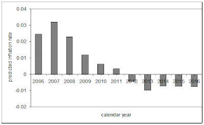
Figure 9. Predicted inflation rate for the period between 2006 and 2016.

Several months ago we presented the same graph with actual inflation readings in this blog:Sure - disinflation continues

Sure - disinflation continues ...

Mark Thoma at "Economists'view" informs us that inflation has been falling for a while and is not going to stop the descend despite many worries. Well. we predicted this outcome 5 years ago [1, 2]. Moreover, the next stage is a deflationary period, also predicted and confirmed many times [3].

Below is the most recent figure with the 1.1% GDP deflator reading in 2009 from my monograph "Deterministic mechanics of pricing". It is only 2 years before the overall price (GDP deflator) will sink below the zero line. ( The original prediction was obtained in 2005 and has been showing an excellent predictive power since.)

Time to buy Treasuries

A deflationary period is coming. As we wrote in 2006, deflation should start in 2012. Some funds (Pimco, for example, as Bloomberg reports) are getting prepared to these poor times. Do not miss the quick start and re-visit our old paper for the prediction of the deflationary period lenght:

Inflation, unemployment, labor force change in the USA
Ivan O. Kitov
Abstract

A model is developed linking the measured inflation (consumer price index or GDP deflator), unemployment and change in labor force. During the last twenty-five years, unemployment in the USA has been a lagged linear function of inflation. In turn, inflation has also been a lagged linear function of relative change in labor force with time. The lag is currently three years. Only a small decrease in labor force participation rate is currently observed in contrast to a strong increase between 1965 and 1990. According to the indicated relationship, the well-known stagflation period clearly resulted from the lag: the sharp increase in inflation coincided in time with the high unemployment induced by the high inflation period two years before. One can predict the unemployment rate in the USA in the following two years within the accuracy of inflation measurements. For example, the end of 2005 is a pivot point from a period of decreasing unemployment to one of moderate growth from 5% in 2005 to 6% in the middle of 2008. Starting in 1960, cumulative values of the observed and the model predicted unemployment are in agreement with the lag between inflation and unemployment. Inflation is defined by a lagged linear function of rate of change in labor force. The observed and predicted inflation almost coincide for the last forty years of annual measurement values, smoothed by a five-year wide moving window curves and as cumulative curves as well. Deviation of the curves before 1960 can be explained by a degraded accuracy of the measurements. A severe decrease in the rate of change of labor force is expected after 2010. This drop can potentially induce a long-term deflationary period. The same effect has been observed for Japan starting in 1990. There are numerous implications of the results for monetary and social policy-makers. The most important is an absence of any means to control inflation and economic growth except though a reasonable labor policy. In addition, some urgent measures are necessary to prevent the start of a deflationary period in 2010-2012.

CPI components in Japan: Medical care and education

As we discussed many times in this blog, Japan has an eternal problem with deflation. The headline CPI and its components are on a long-term decline. It will continue another 40 years because the level of labor force in Japan has been and will be decreasing in line with the ageing and overall depopulation. Today, Japan Statistics released an estimate of the consumer price index for August 2009 - http://www.stat.go.jp/english/data/cpi/1581.htm.

It is instructive, that the only two components (from ten), which did not suffer annual decrease, are the medical care and education. This is in agreement with the extraordinary high rate of growth in both these components in the USA .

Despite the surging prices for medcare and education, the US is awaiting the fate of Japan - a longer deflationary period since 2012.

Deflation in the United States starts in 2012

Notice that this predicition was made in 2005, i.e. seven years in advance. It was publsihed in 2006 and was downloaded around 500 times so far: http://logec.repec.org/scripts/paperstat.pl?h=repec:inq:inqwps:ecineq2006-28

It seems that the economic profession made a good brainwashing of the interested audience, if people do not believe own eyes when see very high correlation, but subconsciously believe in the absence of determinism in economic evolution. Even the presence of cointegrating relations between inflation and the rate of labor force change proved by the Johansen and Engle-Granger (Kitov, I., Kitov, O., Dolinskaya, S., (2007). Inflation as a function of labor force change rate: cointegration test for the USA, MPRA Paper 2734, University Library of Munich, Germany, http://mpra.ub.uni-muenchen.de/2734/01/MPRA_paper_2734.pdf) tests are neglected.


This post repeats major elements of the complete working paper available at the RePEc:

Kitov, I., (2006). Exact prediction of inflation in the USA, MPRA Paper 2735, University Library of Munich, Germany, http://mpra.ub.uni-muenchen.de/2735/01/MPRA_paper_2735.pdf

Abstract
A linear and lagged relationship between inflation and labor force growth rate has been recently found for the USA. It accurately describes the period after the late 1950s with linear coefficient 4.0, intercept -0.03, and the lag of 2 years. The previously reported agreement between observed and predicted inflation is substantially improved by some simple measures removing the most obvious errors in the labor force time series. The labor force readings originally obtained from the Bureau of Labor Statistics (BLS) website are corrected for step-like adjustments. Additionally, a half-year time shift between the inflation and the annual labor force readings is compensated. GDP deflator represents the inflation. Linear regression analysis demonstrates that the annual labor force growth rate used as a predictor explains almost 82% (R2=0.82) of the inflation variations between 1965 and 2002. Moving average technique applied to the annual time series results in a substantial increase in R2. It grows from 0.87 for two-year wide windows to 0.96 for four-year windows. Regression of cumulative curves is characterized by R2>0.999. This allows effective replacement of GDP deflation index by a “labor force growth” index.
The linear and lagged relationship provides a precise forecast at the two-year horizon with root mean square forecasting error (RMSFE) as low as 0.008 (0.8%) for the entire period between 1965 and 2002. For the last 20 years, RMSFE is only 0.4%. Thus, the forecast methodology effectively outperforms any other forecasting technique reported in economic and financial literature. Moreover, further significant improvements in the forecasting accuracy are accessible through improvements in the labor force measurements in line with the US Census Bureau population estimates, which are neglected by BLS.

Key words: inflation, labor force, forecast, the USA
JEL Classification: E3, E6, J21

Introduction
It has been found that inflation in the USA and other developed countries is a linear and potentially lagged function of the growth rate of labor force level (Kitov, 2006a). In the largest developed economies, this relationship has different coefficients and lags. In Japan, Germany, the UK, and some other European countries, there is no clear delay between labor force change and inflation, i.e. the two economic variables evolve synchronously (Kitov, 2006b; 2006d). In the USA and France, however, labor force change leads inflation by two years (Kitov, 2006d). The two-year lag can be easily obtained from annual readings, smoothed and cumulative curves of the labor force growth rate and inflation measured in the countries. Thus, the labor force measurements in the USA and France could be used for forecasting inflation at a two-year horizon.
The leading role of labor force change observed in the USA and France evidences that the change is the driving force behind inflation. The smoothed and cumulative curves obtained for the two variables are in excellent agreement during the period starting in the early 1960s in both countries. Unfortunately, the agreement deteriorates further in past. Such degradation is partially induced by a critical reduction in the accuracy of relevant measurements. Even definitions of labor force and inflation were quite different before the 1960s, as described in technical documentation provided by the US Bureau of Labor Statistics (BLS, 2002).
We do not focus here on the uncertainty in the measurements in the 1950s and before. Instead, our attention is concentrated on the improvement of the US labor force measurements, which have been carried out during the last forty five years. Raw data available at the BLS website (http://www.bls.gov/) is characterized by a number of adjustments and revisions, which cannot be treated as appropriate ones in the framework of the linear relationships between inflation and labor force change rate. Therefore, an assessment of the artificial spikes forced by BLS in the raw data is fulfilled and some corrections are carried out for obtaining a more consistent time series.
The corrections applied to the labor force readings have a great impact on the performance of the linear relationship. This paper documents progressive improvements in standard statistical estimates of the relationship with increasing accuracy of the labor force measurements. In addition, predictive power of the relationship is assessed for various periods, as routinely used in the forecasting literature.
There are just few papers devoted to inflation description and prediction we refer to. Reasons for that are obvious. Inflation models include autoregression as an almost inevitable component. The relationship under study includes no past or future inflation values, no variable representing real economic activity such as unemployment or output gap, and no monetary or financial parameters such as M3 aggregate and interest rates. Instead, the relationship relates inflation to only the change in the number of people who have an intention to obtain a paid job or its equivalent. Hence, there is almost nothing inherited by the relationship from the mainstream economic, econometric, and monetary models of inflation. Results of the study are presented in six sections. First section briefly describes the concept of the labor force induced inflation and empirical coefficients obtained for the USA. GDP deflator is used as a measure of inflation. The deflator is considered as the most robust and accurate variable representing inflation as a real phenomenon because of its inherent relation to the entire economy. An implicit but principal assumption of the concept under development is that all economy-wide variables are related to population-wide quantitative characteristics including entire labor force. Hence, such measures of inflation as CPI and CPE are not appropriate because of their limited population relevance. The variables represent some population sub-ensembles not population as a whole. In statistical physics or thermodynamics, fluctuations in such sub-ensembles are not representative on the entire ensemble level. Following this observation, we do not consider CPI and CPE in the study as potentially misleading variables.
Second section details the adjustments applied by the US BLS to the raw labor force measurements for the period starting from 1960 (BLS, 2006). Several step adjustments of the labor force level introduced by BLS in the annual readings are smoothed. A simple procedure is applied - the step adjustments are distributed proportionally over previous years depending on the period when the changes were accumulated.
Section 3 elaborates on the BLS adjustment applied in 1996 to the labor force readings between January 1990 and December 1993. A “regular” correction applied to the annual values does not help in this case. The 1990 difference between the observed and predicted inflation values is so large that it substantially biases overall statistics. To reveal the reason for the discrepancy the Census Bureau measurements of civilian population (CP) are used. A prominent spike in the civilian nonistitutional population (CNP) increment is reported by BLS for 1990. The spike is not supported by the CB population estimates for the same year. The increment values in both time series are in a good agreement, however, during the entire period between 1980 and 2000 except 1990. The spike is also removed from the original data to fit the postcensal measurements of civilian population. Usage of the intercensal population estimates might provide further improvements in the CNP estimates made by BLS.
Linear regression analysis in Section 4 provides quantitative estimates for the agreement between the observed and predicted inflation values. The labor force readings are used as a predictor. A number of corrections of the labor force estimates is fulfilled and corresponding improvements in the regression results are reported. The original labor force readings for the period between 1965 and 2002 provide a benchmark. The interval selected allows avoiding effects of the labor force data with high uncertainty before 1960 and those of the data after 2002, which are prone to further revisions. In the benchmark case, R2=0.62 and standard deviation is 1.5%. The best corrected labor force time series provides an increase in R2 up to 0.89 and decrease in standard deviation to 0.8%. Further improvements are feasible if to refine the historical labor force data in line with the CB population estimates and to revise the CPS procedures.
Section 5 presents the results of the regression analysis in terms of forecasting. Prediction is a straightforward application of the relationship between inflation and labor force change, at least in the USA. The two-year lag provides a powerful tool for the inflation forecast at the two-year horizon with no extra efforts as compared to the regression. The inflation prediction is intrinsically an out-of-sample one because it uses only past values of labor force. For the entire period between 1965 and 2002, root mean square forecast error (RMSFE) at an annual rate is only 0.8%. Hence, the relationship outperforms modern inflation forecasting models, at least those reported in the literature.
Because of severe problems related to a “break” in the inflation time series around 1984, it becomes a standard way to present forecasting results separately for the periods before and after the break. Our model has no “break” problems due to an outstanding accuracy in the description of the period between 1970 and 1990. The accuracy is a natural consequence of the existence of the objective link between labor force and inflation. Despite the excellent agreement over the entire period between 1965 and 2002, forecasts for two sub-periods, before and after 1984, are also presented to facilitate comparison to other forecasts.
Section 6 concludes and discusses empirical and theoretical advantages of the linear relationship between labor force change and inflation. Empirically, the relationship establishes a strong trade-off between the variables removing any potential discrepancy during measurements. Theoretically, the relationship represents a natural extension of the economic framework, which has been developed by Kitov (2005a; 2005b; 2006a-2006d). The framework links such principal economic variables as GDP, personal income distribution, and now inflation and unemployment to only one endogenous parameter – population. Population counting gives an exact natural number and, thus, provides exact values for the economic parameters.

1. The relationship between inflation and labor force change
The empirical relationship used in the study is obtained and validated by data measured in the USA and Japan (Kitov, 2006a; 2006b). It links together inflation, unemployment, and labor force change rate. An implicit assumption of the model is that inflation and unemployment do not depend directly on real economic growth (Kitov, 2006c).
As defined by the model (Kitov 2006a), inflation and unemployment are linear and potentially lagged functions of labor force change as expressed by the following relationships:

π(t)=A1dLF(t-t1)/LF(t-t1)+A2 (1)
U(t)=B1dLF(t-t2)/LF(t-t2)+B2 (2)

where π(t) is the inflation rate at time t, U(t) is the unemployment rate at time t, LF(t) is the labor force level, t1 and t2 are the time lags between the inflation, unemployment and the labor force, respectively, A1, B1, A2, and B2 are country-dependent empirical coefficients of the linear functions. The coefficients may vary through time for a given country as various measures (definitions) of the studied variables are introduced (Kitov, 2006d).
Linear relationships (1) and (2) define inflation and unemployment separately as functions of labor force change. These two variables are indivisible sides of a unique process, however. The process is the labor force growth, which is accommodated in real economies though two channels. The first channel is an increase in employment and corresponding change in personal income distribution (PID). All persons obtaining new paid jobs or their equivalents presumably change their incomes to some higher levels. There is an ultimate empirical fact, however, that the US PID does not change with time in relative terms (Kitov, 2005b). The increasing number of people at higher income levels, as related to the new paid jobs, leads to a certain disturbance in the PID. This over-concentration must be compensated by such an extension in the income scale, which returns the PID to its original density. The income scale stretching is called inflation (Kitov, 2006a). The mechanism responsible for the compensation and the scale stretching has some relaxation time, which effectively separates in time the source of inflation, i.e. the labor force change, and the reaction, i.e. inflation itself.
The second channel is related to those who failed to obtain a new paid job, i.e. to enter the employment. These people do not leave the labor force but enter unemployment. Effectively, they do not change the PID because they do not change their incomes. So, the total labor force change equals the unemployment change plus employment change, the latter process to be easily expressed through inflation. In the case of a "natural" behavior of an economic system, proportion between unemployment and inflation is retained through time and the linear relationships hold separately. There is always a possibility, however, to fix one of the two variables. For example, central banks are able to fix inflation by some monetary means. Such a violation of the natural behavior will undoubtedly distort the partition of the labor force change – the portion previously accommodated by inflation will be redirected to unemployment. To account for this effect one should to use a generalized relationship as represented by the sum of relationships (1) and (2):

π(t)+U(t)= A1dLF(t-t1)/LF(t-t1) +B1dLF(t-t2)/LF(t-t2)+A2+B2 (3)

Equation (3) balances labor force change, inflation and unemployment, the latter two variables potentially lagging by different times behind the labor force change. The importance of this generalized relationship is demonstrated in (Kitov, 2006d), where the case of France before and after joining the European Monetary Union is analyzed.
For the USA, there is no need so far to apply relationship (3) because corresponding monetary policies do not change the natural partition of labor force change, as observed since the late 1950s. For the USA, A1=4, A2=-0.03, t1=2 years (GDP deflator as a measure of inflation), B1=2.1, B2=-0.023, t2=5 years. Figure 1 compares observed and predicted inflation (annual and cumulative values) as obtained for the USA by Kitov (2006a).
Negative constant A2 makes a permanent increase in labor force of great importance for avoiding deflationary periods. Population growth rate of 0.01 to 0.015 per year, as observed in the USA during the last twenty years, completely compensates the effects of the negative term A2. With the boomers' retirement, however, the labor force growth rate will decelerate starting from 2005.
For Japan, A1=1.77, A2=-0.003, t1=0 years (GDP deflator as a measure of inflation) (Kitov, 2006b). The labor force change rate measured in Japan is negative since 1999 and corresponding measures of inflation, GDP deflator and CPI, are negative as well. There is no indication of any recovery into the positive zone any time soon if to consider the decrease in working age population and participation rate as observed from 1999.
The relationship demonstrates an excellent performance over time and countries. At the same time, there was no formal statistical assessment done for the relationship in the previous papers. Therefore, the relationship is statistically assessed below in order to demonstrate the improvements obtained when the largest errors are removed from to the labor force time series. The errors are discussed in the next two sections.

2. The labor force measurements and adjustments
Results of the labor force measurements are published at a monthly basis by the US Bureau of Labor Statistics (BLS). The readings are obtained during the monthly Current Population Surveys (CPS) conducted for BLS by the US Census Bureau (CB). Details of the CPS definitions, methods and procedures are presented in technical documentation (CB, 2002a; 2002b). Briefly, about 60,000 scientifically selected households compile a sample representing civilian non-institutional population as a whole and are surveyed every month at a rotational basis. All interviewed persons above 15 years of age have to answer a number of questions related to their current labor status. The labor status is one of the following three: in the labor force, i.e. employed or unemployed (not employed but available for a paid job immediately), not in the labor force. Figures in given age-sex-race groups obtained in a survey and corrected for the number of non-interviewed due to various reasons are projected to the entire population using some specific weights related to so-called population controls. The weights reflect the fact that the distribution of the population selected for the sample may differ from that for the population as a whole.
Therefore, the labor force readings obtained in the CPS are characterized by two intrinsic types of uncertainty related to the measurements of the labor force and the total population estimates/counts, respectively. Labor force, as an economic variable, has a long history of changes in definitions, estimation procedures and methodology as documented in (BLS, 2003; 2006).
The CB population estimates used by BLS also undergo some adjustments and revisions between decennial censuses according to new information about birth and death rates and international migration. Decennial censuses in the USA reveal large “errors of closure” (CB, 2002a), i.e. the discrepancy between the estimated and the census counted population. The errors are age-sex-race dependent and are as large as several per cent. For example, the undercount of the population between 25 years and 34 years of age reached 5.92% in the 2000 census, i.e. instead of the estimated 39.9 million 43.2 million was counted. Thus, when using the population controls in the labor force estimation procedure, one has to bear in mind that the population controls are exposed to multiple revisions and modifications in line with new enumeration and other estimates.
The changes in labor force concepts, definitions and methods induce uncontrollable (but, hopefully, not large) errors in the labor force estimates made in the USA during the last 50 years. Not every change in the CPS questionnaires and practice of the CPS can be extrapolated back in past because of the absence of relevant information. In addition to these immeasurable changes, there are adjustments which are applied to the labor force time series and can be described quantitatively.
Figure 2 summarizes the changes in the labor force level during the last 45 years. In 1962, the labor force was decreased by 200,000 according to the population data obtained in the 1960 census. Here we first meet an example of the labor force level adjustment. Despite an obvious cumulative character of the population estimate error, the adjustment is applied to only one year, i.e. in a way, which artificially introduces a step in the labor force level. The US Census Bureau proportionally distributes the error of closure over the ten years preceding the censuses (CB, 2002a). The population controls used in the estimation of the labor force are adjusted by BLS impulsively, however.
In 1972, an adjustment related to the 1970 census was introduced and the total population was increased by about 800,000. The labor force level was increased by only 300,000, however, that corresponds to different labor force participation rates characterizing different age-sex-race groups used in the surveys.
An important modification was introduced in 1974. The CNP has been estimated by an “inflation-deflation” method since then. BLS states that the modification had no impact on the labor force level, however, in contrast to the next year when about 76,000 refugees arrived from Vietnam. The labor force was also increased. This is an example of a real step change in the labor force level. The newcomers entered the labor force at once. No correction for this event is made in the labor force estimates.
In January 1978, a 250,000 increase in the labor force was introduced as resulted from an expansion of the survey sample (the number of the sample areas was increased from 461 to 614) and revisions of the estimation procedure. A series of changes in methods and procedures between 1979 and 1985 did not result in any important revision of the labor force level. In 1985, “the population controls used in the second-stage ratio adjustment method were revised” (BLS, 2006) that led to an about 350,000 increase in the labor force.
Almost the largest labor force positive revision was implemented in 1994. The CNP for 1990 was increased by 1,100,000, the employment level by 880,000, and the unemployment by 175,000. This adjustment was related to the 1990 census and distributed by BLS over the period from January 1990 to December 1993. The labor force level was revised up by about 1,000,000 in January 1990, however, introducing a very high step in the time series.
In 1997, the labor force level was increased by 320,000 due to the new population controls related to the demographic updates for the number of international migrants. New composite estimation procedures introduced in 1998 resulted in lower estimates of the civilian labor force. It is not clear what effect it had on the years before 1997, but in 1997 the labor force was reduced by 229,000. A minor positive labor force change of 60,000 introduced in 1999 was related to updates of immigration information.
Since 2000, several major changes have been introduced into the CPS. The changes reflect results of the 2000 census enumeration, introduced by a 1,600,000 positive labor force level correction, and a higher population growth rate between 2000 and 2003, additional 900,000 were distributed month by month between January 2000 and December 2002. Total increase accumulated in 2000 reached 1,900,000. An upward adjustment by 614,000 was introduced into the labor force in January 2003.
In January 2004, the labor force was decreased by 440,000, however, to reflect new immigration estimates for the period between 2000 and 2004. So, frequency and amplitude of the adjustments has been progressively increasing in the twenty first century as presented in Figure 2. During the 1960s and 1970s, there were only minor and seldom changes.
The detailed description of the BLS revisions evidences that the reasons behind the adjustments are clear and valid. At the same time, except the case of the Vietnamese refugees, the labor force level errors compensated by the adjustments were accumulated during periods longer than one year. This makes the step adjustments to introduce some additional errors in the labor force estimates. The errors are especially important to understand and remove in the following regression analysis because the step level adjustments create spikes in corresponding growth rates as the first differences, which substantially affect results of such a least squares based procedure as linear regression.
There are two simple ways to reduce the influence of the step adjustments. The first is to subtract the adjustments from the official estimates. This would remove the artificial steps from the time series. This approach has a substantial deficiency, however. It contradicts the observations: both the census enumerations of the total population and in population subgroups. Also it excludes advances in the labor force measurement procedures which reduce uncertainty in the readings.
Another way is to distribute the step adjustments over corresponding periods. For example, the adjustments associated with decennial censuses were apparently accumulated during the entire period between corresponding censuses. The proportional distribution applied by the Census Bureau to the civilian population estimates would be a reasonable first approximation. One should bear in mind, however, that actual distribution over years differs from its simplest representation and some years between censuses are potentially characterized by higher or lower than average changes. Therefore, using the proportional distribution one may reduce variation in the labor force measurements but can not recover the actual pattern.
Figure 3 illustrates the proportionally distributed corrections designed to smoothing the BLS step adjustments. The corrections effectively reduce variance in the labor force increment values as Figure 4 demonstrates. There is one year, however, which does not show any improvement. It deserves a special consideration.

3. The problem of 1990
In the previous Section, we corrected the labor force estimates for the step revisions. The revisions are recognized by BLS as leading to the noncomparability of labor force levels (BLS, 2006). So, the steps are artificial and our corrections resulted in several improvements expressed in the smoothness of the modified labor force change rate curve compared to the original one, especially between 1970 and 1990.
There is a significant outlier, however, in 1993. The predicted inflation still falls to negative values and differs from the observed value by almost 3.5%. This discrepancy is of critical importance for the linear relationship between inflation and labor force change. It is clear that the larger is the difference the lower is the confidence that the relationship is valid: large changes are usually better measured in relative terms and provide major input into statistics of fit. If large changes are not well described by a model, common sense and statistics both evidence the failure of the underlying concept. Due to the importance of the 1993 outlier for the concept, we study this case in more detail.
First, I requested BLS to give an explanation of the sudden drop in the labor force change rate observed in 1991. In a personal communication, explanation just referred to a recession observed between July 1990 and March 1991. Supposedly, the recession led to a decrease in the employment growth rate and corresponding drop in the observed labor force change rate. If the explanation is valid, it denies the approach because the reason or driving force behind inflation is not the labor force change but business cycles.
The revisions for the years between 1990 and 1994 are well documented by BLS (2003, 2006). There was only one step adjustment applied in 1990, when the labor force was increased by 1,055,000. The step increase was accounted for in the previous Section but the correction did not give any significant improvement. In any case, there is no inconsistency in the revisions from the BLS side. But it is only one side of the story.
BLS borrows its population control numbers from the Census Bureau and uses them in somewhat independent way. To obtain the labor force estimates, BLS multiplies civilian noninstitutional population by participation rate. The latter value is obtained through the monthly CPSs and characterized by a relatively high accuracy. At least the participation rate values are consistent through time. The CNP is an estimated (enumerated) parameter, however. The largest revisions are usually applied after decennial censuses. The closest census to 1991 was in 1990. So, a hypothesis easily arises that BLS used some earlier and inaccurate revisions to the population controls, which later were improved by the Census Bureau.
The Census Bureau provides two sets of population estimates for the period after 1990. The first estimate of civilian population is obtained between censuses and is called a postcensal estimate. This estimate uses all available contemporaneous information to assess population changes induced by births, deaths, and net migration. The second estimate is based on enumerated values obtained in censuses and is called an intercensal estimate for years between the two censuses. The second estimate is characterized by a superior accuracy because it is based on actually counted numbers.
Both population estimates were obtained from the CB website. There is a principal difference between the CNP used by BLS for the population controls and the civilian population presented by CB. But the latter represents a good approximation of the former if to consider annual increments not levels. Figure 5 displays the annual increments in the BLS CNP and increments in the civilian population of 16 years of age and over as obtained from the post- and intercensal estimates. All the curves practically coincide between 1980 and 1989 with just minor deviations of the CNP increments from those of the civilian population. The latter is the same for the post and intercensal estimates. In 1990, a spike is observed in the BLS CNP which is demonstrated neither by the intercensal nor by the postcensal civilian population estimates. This spike actually represents the BLS step adjustment applied to the CNP in 1990. The increments in the postcensal estimates practically coincided with those in CNP for the rest of the years. Hence, the postcensal estimates is probably the source of information for the CNP estimates conducted by BLS. The intercensal estimates demonstrate consistently higher annual increments resulted from a number of revisions conducted by the Census Bureau after the 2000 census. The revisions compensate for the “error of closure".
Hence, the sudden drop in the labor force change rate in 1991 is induced by the 1,000,000 overestimate in the CNP increase during 1990. If the participation rate is determined accurately (~66%), the labor force estimate for 1990 is positively biased above its actual value and the estimate for 1991 is not biased. As a result, the difference between the 1991 and 1990 labor force estimates is below its actual value by approximately 660,000. One can use the intercensal civilian population curve for a better estimate of the labor force change in 1990 and 1991. The curve definitely shows that the annual increment values grew gradually between 1990 and 1992.
One can apply the CB estimates of civilian noninstitutional population increment for the entire period after 1990 instead of those used by BLS. It is a sophisticated procedure, however, which includes re-estimation of participation rates in numerous age-sex-race groups and we leave this problem with BLS. For the purposes of our study, we just distribute the excess of 660,000 over the period between 1990 and 1992, as the CB intercensal estimate shows. Figure 6 illustrates the smoothness of the obtained distribution of the labor force increment between 1985 and 2000 compared to that for the original distribution. There is no deep trough near 1990 any more.

4. Regression
In hard sciences, statistical estimates usually do not provide additional confidence in results if some curves literally coincide as the cumulative curves in Figure 1. Formally, one can apply some statistical techniques in order to assess the residual level of uncertainty related to the curves. The reason for the statistical estimates of uncertainty is not to report them as they are but to develop some instrumental and/or theoretical approach to decrease the attained level of uncertainty. This is a standard procedure in hard sciences: to measure – to estimate degree of uncertainty – to develop a new approach to improve accuracy of the measurements, instrumentally or theoretically – to measure at the new level of accuracy, which can potentially distinguish between accepting and denying the model. An implicit assumption behind the procedure is that real empirical relationships can be potentially evaluated with a progressively lower level of uncertainty improving our understanding of real processes behind the relationships. (We do not consider here the uncertainty principle, which limits accuracy of simultaneous measurements of some quantum variables.) Levels of uncertainty related to such physical relationships are usually estimated as the discrepancy between predicted and observed values. This approach often makes any additional statistical estimates unnecessary. A researcher has usually a good reason to relate the observed discrepancy to corresponding measurement errors if the observations and predictions do not violate physical laws.
In economics, the feedback between measurement accuracy and theoretical analysis is much weaker. There are few recommendations on the level of measurement accuracy necessary to resolve specific economic problems in a majority of economic papers. Even those devoted to measurement accuracy usually do not link the evaluated level of uncertainty to solution of principal economic problem. Accuracy problems are left to measuring agencies with no specific criticism of the applied definitions, procedures, practices, etc.
Replacing the improvements in measurement accuracy as an ultimate demand of evolving economic theory, statistical analysis becomes a backbone of economics as a science. Such an approach is considered as an appropriate one because of a strong and consolidated opinion among economists that real economy is a stochastic and unpredictable process. Thus, only statistics is able to provide an adequate formal description of economic processes. In other words, there are no other links between economic variables except statistical ones. Because of the absence of predetermined and unambiguous links between economic variables, there is no specific need to improve accuracy of economic measurements. One can not distinguish between random errors in the measurements and random behaviour of economic variables. Statistically, they maybe treated as identical. As a result, standards of economic measurements are driven not by demands of science itself but by internal conventions developed in measuring agencies and funding. The latter is always a critical issue, but in the absence of reliable objective relationships between economic variables, there is no rule how to distinguish the most important measurements for the overall progress of economic theory.
I am also sure that real economy is a stochastic process. But not an unpredictable one! Driving forces behind numerous economic variables – this is the real source of stochastic behaviour. The driving forces are governed by a large number of natural processes and events, which effectively introduce a stochastic component into the forces. However, many macroeconomic variables are completely defined by the forces with some time lags providing a better opportunity to reveal the forces and to predict the variables.
For example, inflation is completely controlled by relative growth in labor force, as claimed in this paper. Relationship between the variables is linear and lagged. Thus, inflation is a random variable to the extent the labor force growth is random. Labor force change rate depends on a variety of financial, fiscal, social, demographic, climatic, and historical processes. But labor force level can be measured with any desirable accuracy if a strict definition is given. Thus, the aim of this Section is to demonstrate that inflation can be also predicted exactly with improvements in the accuracy of labor force measurements.
As statistical inferences play an important role in the current economic thinking it would be reasonable to provide some results of a standard regression analysis. This allows translation of the findings into “econometric language” for better understanding of the link between labor force and inflation. Regression analysis does not make the findings about the link more convincing by itself, with the most actual future problem being a substantial improvement in the accuracy of the labor force measurements.
Inflation is chosen as a dependent variable and labor force change rate is the predictor. The period between 1965 and 2002 is selected for balancing between sample length and uncertainty in corresponding measurements in the USA. Before 1965, the large variations in the labor force annual increment (see Figure 1) evidence some measurement problems. After 2002, the labor force measurements are prone to further (and potentially severe) revisions, i.e. any regression results would be just temporary. So, the length of the period is 37 years with 38 annual readings. Such a choice does not indicate that we consider the studied relationship as not working before 1965. It should be valid before 1965, to some point in the past which practically can not be determined due to data related problems. After 2002, the relationship is also valid and will be valid before economic behavior of the US population and institutions changes in some dramatic way.
The annual readings of inflation are regressed against the predicted values of inflation as obtained using relationship (1) with the coefficients described in the text and in Kitov (2006a) and the measured rates of the labor force change. Table 1 lists some principal results of the regression. The regression coefficient is 0.763 (0.099) and R2=0.62. Thus, about 60% of the inflation variability is explained by the linear relationship. Here we have to mention that the labor force readings are shifted by two years ahead to compensate for the observed time lag. Standard error of the prediction with the linear lagged relationship is 0.015 (1.5%). P-value and t-statistic associated with the regression coefficient are given for additional confidence.
As discussed in Kitov (2006a) and above, the labor force measurements are characterized by a significant scatter. The relatively low R2 obtained in this first regression experiment indicates that almost 40% of the labor force variance is potentially related to the measurement error with the residual 60% explaining the variance of the inflation. As found in Sections 2 and 3, the original labor force readings are strongly biased by the step adjustments carried out by BLS. The reason why we have smoothed the original data and introduced a special correction to the 1990 reading is to make the measured values closer to actual or exact ones. Whether the goal is achieved may be demonstrated by a comparison of the results of regression analysis using the original BLS labor force readings to those obtained with the corrected values. Table 1 answers the question quantitatively. The regression coefficient for the corrected labor force readings for the same period is 0.890 (0.085) with R2 =0.75. This result evidences a significant improvement in the explanation of the inflation variation by the labor force change rate if the latter is just corrected for the simplest and obvious errors introduced by BLS. Apparently, the original labor force measurements include some more errors associated with changes in definitions, procedures, practices, etc. These errors are poorer described and understood, but a scrupulous researcher might reach better regression results conditional on time and efforts invested. We do not go further in our efforts to recovering unbiased signals from the original data.
Another significant improvement can be achieved by a trivial time shift of the labor force estimates by half a year. As discussed in Kitov (2006a), the labor force annual readings are obtained by a weighted averaging of monthly measurements with corresponding seasonal adjustment. Obviously, these average values are closer to the midyear monthly estimates than to the end-of-year monthly values. Therefore, the annual readings are expected to better describe the July through June changes in the labor force rather than the January through December changes. The easiest way to compensate for the time shift between the inflation and labor force measurements is to recalculate the average values for the corresponding shifted periods with December in the middle, i.e. July through June of the next year. Table 1 provides the results of the regression analysis as obtained for the newly averaged labor force values marked as “July-June dLF/LF”. For the original data series, i.e. the one not corrected for the step adjustments, R2 increases from 0.62 to 0.73, and standard deviation decreases from 0.015 to 0.013. Thus, there is a difference in the explanatory power between the original and half-year shifted data series. The latter is superior. There is also a lesson for researchers using original economic data sets. Sometimes even a half-year shift results in further improvements in statistical description.
A different way to achieve a half-a-year shift in the labor force series is the averaging of two neighboring annual values. This procedure effectively makes the center of the two-year wide periods, i.e. December, to represent the averaged readings and introduces additional noise suppression. Table 1 lists regression results for two cases: the half-year shift applied to the original time series “dLF/LF+1/2 year shifted LF” and the shift applied to the corrected values “dLF/LF (corrected)+1/2 year shifted LF”. (Further in the text, “1/2 year shift” means averaging of two neighboring values.) In both cases, the dependent variable is the annual inflation. R2 increases to 0.807 and 0.845, and standard deviation decreases to 0.011 and 0.010, respectively. Figure 7 displays the observed inflation values and those predicted with the corrected and shifted labor force estimates. In fact, there is almost nothing left to explain with the annual readings considering the noisy measurements of the labor force and potential measurement errors in the GDP deflator values.
Smoothing by moving average is a simple and effective way to suppress random noise by destructive interference. Efficiency of such a method when applied to the labor force and inflation measurements was demonstrated by Kitov (2006a). Seven-year moving average provided an outstanding similarity of the smoothed curves - observed and predicted ones. In this paper, a shorter time series is analyzed with only 38 observations. This makes the seven-year window too wide compared to the total length.
At first, averaging by two-, three-, and four-year wide moving windows was carried out using the corrected labor force annual readings. Then the “1/2 year shift” procedure was applied to the averaged values, i.e. an additional weighted averaging. Then the annual inflation readings were regressed against the predicted values. Table 1 summarizes corresponding information. Averaging in two-year wide moving windows with one year step provides a better description of the annual inflation readings (R2=0.866) compared to that obtained using the corrected labor force values (R2=0.752) and the half-year shifted original values (R2=0.807). Standard deviation is only 0.009 (0.9%), i.e. potentially less than the accuracy associated with the inflation measurements. However, the best result is achieved by the three-year window averaging with R2=0.894 and standard deviation of 0.008. The extension of the moving window to four years provides additional improvement neither in R2=0.893 nor in standard error – 0.008. Such a result is not an unexpected one because of the two-year lag between the inflation and labor force change. Labor force readings around the defining year may introduce some noise suppression due to effects of serial correlation intrinsic to the labor force measurements but do not bring any actual information in addition to that already available for the defining year. When extended beyond some critical width, the averaging window includes more and more information related to different years, what is pure noise for the defining year. As a result, correlation between the inflation and the labor force deteriorates.
The regression of the observed and predicted values of inflation averaged in two-, three-, and four-year wide windows with one-year step provides an additional improvement. Table 1 evidences that corresponding R2 values are consequently increasing: 0.897, 0.941, and 0.963. One can consider the improvements as an indication of the expected noise suppression. Figure 8 depicts the predicted and observed curves for the latter case with the error in 1990 intentionally left to demonstrate its influence on the deviation of the predicted curve.
The last two rows in Table 1 are devoted to the cumulative curves. In practice, the curves obtained by a progressive summation of the inflation values, the measured and predicted ones, starting from 1965 (and 1963 for the predicted series) are just routinely constructed indices. The curves look identical with just minor deviations induced by such errors as we discussed for the 1990 civilian noninstitutional population value. Regression confirms the visual identity. R2 reaches 0.999 for the GDP deflator and 0.998 for CPI inflation. Standard deviation is 0.014 and 0.026, respectively.

5. Forecasting inflation
Forecasting inflation is the principal task for monetary authorities. In developed countries, there are several approaches elaborated during the last half-century. It would be not an exaggeration to divide bankers and economists involved in the forecasting process into two principal groups, as introduced by Mankiw (2005), “technical” forecasters and “scientific” ones. There is no any unique concept or approach recognized as a superior one across the groups and inside the groups as well. In practice, technical decisions (or “engineering” in the Mankiw’s classification) are more popular than scientific ones. (Here I would like to notice that no engineering is possible without science.) This slight superiority is not justified by any better result in forecasting relative that obtained by the scientific community. The superiority is dictated by an easier access to monetary power (Mankiw, 2005) and consideration of the fact that somebody has to make principal decisions in the situation of the absence of any hard science. The relationship between inflation and labor force provides all necessary means for precise forecasts with potential improvement depending on accuracy of labor force measurements.
To some extent, current inflation forecasting for monetary purposes can be described as a common sense selecting between the tools available and experiences. That is why personal influence is so important in actual practice of monetary authority - there is no best description of inflation processes - just numerous competing. Moreover, as stated in the modern literature on inflation forecasting- Stock&Watson (1999; 2005), Atkeson&Ohanian (2001); Canova (2002), Hubrich (2003), Ang, Bakaert, and Wei (2006), among others, a naïve approach based on the assumption that tomorrow’s inflation will be equal to the one observed today is superior during the last twenty years to almost any scientific approach based on information related to previous behavior of inflation and other economic and financial variables. In fact, those approaches, which are superior to the naïve one, are very close to it and often are volatile ones. They will probably loose their predictive power soon (Stock&Watson, 2005). Hence, to be a great forecaster one needs only to know current inflation value and maybe have some historical experience to be ready for a “pivot point” when inflation will start to deviate from its current “moderate” behavior.
There is no strict scientific knowledge behind these “engineered” forecasts, however. This makes long-run forecasts to be very poor, as it was observed during the 1970s and 1980s. Both naïve and “engineered” approaches failed to explain sudden peaks and disinflation. There is no simple candidate parameter, except inflation itself used in the naïve or autoregressive form, which could potentially explain historical readings of inflation through time and countries. Many parameters provide temporary and country specific improvements over the AR-type models, however.
The approach we present resolves these problems. It does not use autoregressive properties of inflation, i.e. there is no rational expectation implied, perfect or imperfect one, what is a common feature for the Phillips curve based models (Rudd&Whelan, 2005). It covers the entire period when relatively accurate labor force data is available for developed countries (Kitov, 2006b; 2006d).
One can describe inflation in the USA with an uncertainty controlled by the accuracy of the labor force survey, as demonstrated in Section 4. Thus, a direct way to improve the current predictive power of the inflation/labor force relationship is available. Only some simple arrangements are necessary. Moreover, one can easily introduce a target value for the inflation uncertainty and link it to the resources available and needed.
According to our concept, inflation forecasting is equivalent to the inflation regression carried out in the previous Section. Standard deviation listed for various regressions is, by definition, the prediction uncertainty for the entire period between 1965 and 2002. In forecasting practice, standard deviation is called root mean square forecast error (RMSFE). This term indicates that forecasted values of inflation are obtained in the framework of out-of-sample approach, i.e. using only past values of predictors. Models explaining inflation, such as the family of Phillips curves, often include past, contemporaneous, and future values of economic parameters (for example, Gali, Gertler, and Lopez-Salido (2001) and Sbordone (2002)) .
The best prediction for the annual readings with RMSFE of 0.008 (0.8%) is obtained in Section 4 using a three-year moving average. Even the annual readings of the labor force with the simplest improvements such as smoothing of the step adjustments and a half-year shift provide RMSFE of 0.096 (0.96%). These values are lower than any RMSFE at the two-year horizon I was able to find in literature for the same or comparable period.
It is practically a standard to make forecasts for periods before and after 1983 separately. To match this standard, the period between 1965 and 2003 was split at the same point. Linear regression is carried out for the separate periods and RMSFE (standard deviations) are computed. Table 2 lists the obtained statistical estimates. The best prediction for the earlier period is characterized by RMSFE=0.011and R2=0.81. It is received using the three-year moving average. Standard deviation of the inflation time series for the same period is 0.023 (first row in Table 2). For the period between 1983 and 2002, the bets prediction is also obtained with the three-year moving average: RMSFE=0.0045 and R2=0.72. Standard deviation for the inflation during this period is 0.009. Stock and Watson (2005) provide a comprehensive list of RMSFE for the periods between 1970 and 1984 and between 1984 and 2004. For the first period, the best RMSFE=1.85%, and for the second – 0.67%.
Our forecasts are made on an annual rate of inflation and at the two-year horizon. In the literature, a quarterly basis is more popular for various reasons. There is only a marginal difference between statistical estimates made for the inflation at an annual and quarterly basis for the period between 1965 and 2002: mean value is 0.042 and 0.041, standard deviation is 0.024 and 0.025, respectively. For the two periods before and after 1983, the difference between the values obtained for the annual and quarterly readings is also of 0.001, i.e. practically negligible.
In addition to the overall statistics, linear regression analysis was carried out at a quarterly rate for the period between 1965Q1 and 2002Q1. Predicted values were obtained by relationship (1) using the annual labor force measurements two years before the predicted quarter, i.e. the average labor force over the four preceding quarters. For the entire period between 1965Q1 and 2002Q1, R2=0.64 and stdev=0.015, i.e. very close to the values obtained at an annual rate for the annual readings of labor force without any correction: R2=0.62 and stdev=0.015. This indicates that the quarterly forecasts from literature and our annual forecasts can be compared without any adjustment. The comparison undoubtedly evidences that predictive power of the relationship between inflation and labor force is superior to any other reported forecasting methodology. Moreover, the relationship is the same for both periods. Values of linear coefficient (4) and intercept (-0.03) are obtained from the entire period between 1965 and 2002. There is no additional adjustment applied to the coefficients when forecasting inflation for a specific time span. In different forecasting models, coefficients, the number of which is usually more than 2, are adjusted to the periods before and after 1983 in order to minimize RMSFE. Even using these additional advantages the models fail to produce a good prediction compared to that the relationship between inflation and labor force easily provides.

6. Discussion and conclusions
The most important conclusion is that inflation can be described (predicted) with a high accuracy, being at the same time a stochastic variable. In the framework of the linear lagged relationship between inflation and labor force change, there is no difference between description and forecast because only past values of labor force are used. Further improvements in the accuracy of inflation forecasts are straightforward and depend only on our capabilities to measure labor force level. Stochastic properties of inflation are entirely defined by those of the labor force. Therefore, inflation as a process is stochastic to the extent the labor force growth is stochastic. If labor force could be controlled by some means, inflation would be also controllable.
Current methods applied by the Federal Reserve Board do not provide any contemporaneous influence on the inflation and potentially affect only the future evolution of the variable to the extent they affect the labor force. Moreover, one can conclude that there has been no change in the methods, at least since the late 1950s, which has affected the observed evolution of inflation, i.e. its link to the labor force change rate. The evolution of the labor force has been affected by different processes, not by the FRB actions, during the period. One can hardly imagine any influence of FOMC decisions on working age population growth rate.
The standard errors of inflation forecast (or RMSFE) obtained using three-year moving averages apparently are the best ones available so far and are superior to any other prediction at the two-year horizon including the Phillips curve, interest rate, monetary aggregates, and survey forecasts. The simplest and obvious corrections applied to the labor force readings resulted in the R2 increase by 0.25-0.40. In addition, the best standard error of prediction has approached 0.8%. Revisions of the labor force estimates through the last forty to fifty years in line with the CB civilian population re-estimates is a natural next step. There should be no artificial steps in the labor force estimates potentially induced by changing definitions and procedures and the population controls should reflect the last revisions made by the CB.
Noise suppression by moving average results in a significant increase of R2 to the level approaching 1.0. The predicted and observed curves are hardly distinguishable when four-year wide moving windows are used. The cumulative curves (or indices) could successfully substitute each other over the entire period with R2=0.9991.
There is a number of negative conclusions one can make considering the results of the analysis. The Phillips curve was not mentioned in the text in any positive sense because it obviously does not exist. There is a link between inflation and unemployment as described by relationship (3), but unemployment or any other variable expressing real economic activity does not affect inflation in the Phillips curve sense. This is not rational expectation, supply shock and real economic activity what determines evolution of inflation. These variables potentially have some marginal effect on the labor force evolution observed in the USA during the last 50 years. So, I would consider the Phillips curve as a dead end in macroeconomic theory.
There is no structural or any other kind “break” around 1984. The changes in the inflation behaviour observed in the 1970s and 1980s are a pure consequence of the accelerated labor force growth associated with the measured participation rate increase (Kitov, 2006a). There were two distinct phases in the participation rate increase separated by a short period of “quietness”. When reached its peak value around 1983, the participation rate effectively stalled at the attained level and has not been changing since then. As a consequence, the labor force has been growing only due to the growth in working age population. This period is known as “Great Moderation” and was possible completely due to the constant participation rate and population growth at an annual rate above 1.0% since 1983.
The “Great Moderation” is currently approaching its natural end. The labor force projections made by various institutions (CBO, 2004; BLS, 2005) undoubtedly indicate a decrease in the participation rate and a decaying growth rate of the working age population. According to the projections, staring from 2010, the annual increase in labor force will be less than 1,200,000 – the value separating inflation and deflation. Hence, a deflationary period is very probable starting 2012 because of the two-year lag between the labor force change and inflation. Similar prediction was given by Kitov (2006a) based on a projection of working age population in the USA.
Figure 9 details the prediction based on the CBO’s projection of the labor force. Currently (2006) inflation undergoes a short-term increase with a peak in 2007 reaching 3.2%. After 2007, a gradual decrease will be observed with the first red figure in 2012.

References

Ang, A., Bakaert, G. and M. Wei, (2006). “ Do macro variables, asset markets, or surveys forecast inflation better?”, FRB Working Paper ?
Atkeson, A., Ohanian, L.E., (2001). “Are Phillips curves useful for forecasting inflation?”, Federal Reserve Bank of Minneapolis Quarterly Review 25, 2-11.
Bureau of Labor Statistics, (2003). “Revisions in the CPS effective January 2003”, http://www.bls.gov/cps/eetech_methods.pdf
Bureau of Labor Statistics, (2005). “Labor force projections to 2014: retiring boomers”, Monthly Labor Review, November 2005.
Bureau of Labor Statistics, (2006). “Employment and Earnings. Household data”, http://www.bls.gov/cps/eetech_methods.pdf
Canova, F., (2002). “G-7 inflation forecast”, EBC Working Paper No 151.
Congressional Budget Office, (2004). “CBO’s Projections of the labor force”, September 2004.
Census Bureau, (2002a). “ Methodology: national intercensal population estimates", http://www.census.gov/popest/archives/methodology/intercensal_nat_ meth.pdf
Census Bureau, (2002b). “The Current Population Survey: Design and Methodology”, Technical paper 63RV, Washington, U.S. Census Bureaus and Bureau of Labor statistics, March 2002. http://www.census.gov/prod/2002pubs/tp63rv.pdf
Gali, J., Gertler, M., Lopez-Salido, D., (2001). “European Inflation Dynamics”, European Economic Review 45(7), 1237-1270.
Hubrich, K., (2003). “Forecasting euro area inflation: Does aggregating forecasts by HICP component improve forecast accuracy?”, ECB Working Paper No 247.
Kitov, I., (2005a). "A model for microeconomic and macroeconomic development," Working Papers 05, ECINEQ, Society for the Study of Economic Inequality.
Kitov, I., (2005b). "Modelling the overall personal income distribution in the USA from 1994 to 2002," Working Papers 07, ECINEQ, Society for the Study of Economic Inequality.
Kitov, I., (2006a). "Inflation, Unemployment, Labor Force Change in the USA". Working Papers 28, ECINEQ, Society for the Study of Economic Inequality.
Kitov, I., (2006b). "The Japanese economy". Available at SSRN: http://ssrn.com/abstract=886663.
Kitov, I., (2006c). "GDP growth rate and population". Working Papers 42, ECINEQ, Society for the Study of Economic Inequality.
Kitov, Ivan, (2006d)." Inflation, Unemployment, Labor Force Change in European countries". (in preparation)
Mankiw, N.G., (2005). “The macroeconomist as scientist and engineer”, manuscript, Harvard University,
http://post.economics.harvard.edu/faculty/mankiw/papers/Macroeconomist_as_Scientist.pdf
Rudd, J., Whelan, K., (2005). “New tests of the New Keynesian Phillips Curve. Journal of Monetary Economics”, forthcoming.
Sbordone, A. (2002). “Prices and Unit Labor Cost: a New Test of Price Stickiness”. Journal of Monetary Economics 49(2), 265-292.
Stock, J.H., Watson, M.W., (1999). "Forecasting inflation," Journal of Monetary Economics 44, 293-335.
Stock, J.H., Watson, M.W., (2005). “Has inflation become harder to forecast?”, manuscript, Harvard University, http://ksghome.harvard.edu/~JStock/pdf/qepd_sw_jmcb_submission_1.pdf

Figure 1. Observed and predicted inflation (GDP deflator). The predicted values are obtained using relationship (1). The upper panel compares annual readings and the lower one – cumulative values. Notice high variation in the labor force annual increments.

Figure 2. Step adjustments to the levels of labor force estimates conducted by the US Bureau of Labor Statistics between 1960 and 2004.

Figure 3. Corrections applied for smoothing the step adjustments in the labor force level shown in Figure 2. The corrections proportionally distribute the adjustments over previous years.

Figure 4. Results of the corrections to the BLS labor force estimates – comparison of the original and corrected increments in the labor force level. A lower volatility is observed except for 1990.

Figure 5. Comparison of the annual increments in the civilian noninstitutional population reported by BLS (CNP BLS) and the annual increments in the civilian population of 16 years of age and over as reported by the US Census Bureau for the postcensal and intercensal estimates.

Figure 6. The labor force increments around 1990 after removing the spike in the 1990 CNP estimate.

Figure 7. Comparison of the measured inflation to that predicted using the corrected labor force estimated and a half-year shift.

Figure 8. Comparison of the observed and predicted inflation time series smoothed by a four-year wide moving window. The original value of the labor force in 1990 is intentionally used in order to demonstrate the influence of the measurement errors on the otherwise excellent agreement.

Figure 9. Predicted inflation rate for the period between 2006 and 2016 according to the CBO’s (2004) labor force projection. A deflationary period starts in 2012.