Political Calculations on recession in 2013

Ironman @ Political Calculations presented a measure which might indicate recession in 2013: the number of publicly-traded U.S. companies acting to cut their dividend payments each month.
A year ago, we presented a different measure showing a hightened probability of recession.
It seems that the change in populaiton is the reason for the companies to cut dividents.

Real GDP per capita in developed countries

Five years ago I published a paper [1] introducing the concept of constant annual increment in real GDP per capita, G(t), as observed in developed countries. In the long run, the GDP growth as a linear function of time:

G(t-t0)= G0+A(t-t0)

where G0 is the initial level of GDP per capita at time t0 in a given country, A is the country dependent increment measured in PPP dollars. Therefore, the rate of growth of real GDP per capita, dG/G, has a decelerating nonlinear trend:

dG/G = A/G

This assumption gives excellent statistical results and explains the evolution of real GDP per capita in developed countries, as also was confirmed in our 2008 paper [2].

Hence, the task now is to track the progress of the economies under study. The figure below presents several important cases, which demonstrate the accuracy of our concept. Since the increment is assumed to be constant, the mean value of the annual GDP increment should coincide with its linear trend (see the paper for details). In reality, the linear regression line is very close to the constant level. In many cases (e.g. France, Italy, Japan), it oscillates around the mean value over time with a small amplitude. The hypothesis of the constant increment looks sound.

Figure. The increment of real GDP per capita vs. real GDP per capita in select developed countries. Thick line – the mean increment. Two solid lines represent two linear trends (also represented by their equations) as associated with the original and population corrected GDP estimates. All data are borrowed from the Conference Board data base (http://www.conference-board.org/economics/database.cfm).

References
[1] Kitov, I., (2006). Real GDP per capita in developed countries, MPRA Paper 2738, University Library of Munich, Germany, http://ideas.repec.org/p/pra/mprapa/2738.html

[2] Kitov, I., (2009). The Evolution of Real GDP Per Capita in Developed Countries, Journal of Applied Economic Sciences, Spiru Haret University, Faculty of Financial Management and Accounting Craiova, vol. IV(1(8)_ Summ), pp. 221-234.

Black Tuesday?

I assume that the closing S&P 500 level of 1183 in October 2010 and its following growth to 1225 in November 2010 is not good news for the US stock market. Figures 1 and 2 update the previous versions published in this blog in September. Both Figures demonstrate that the difference between the predicted and observed curves has been increasing since September.

This observation raises a question on the following events. Our concern about possible repetition of the 1987 fall, if the index would continue its deviation from the predicted trend into October 2010 is on again. So, I see a danger of a severe panic on the stock market. Because Tuesday is a common day for such events, I cannot exclude that one of Tuesdays in the nearest future will end in a return of the observed curves to the predicted one.

There is also a chance that the population estimates underlying the prediction become wrong since September 2010. The methods of population projection and updates used by the Census Bureau are also not well predicted.

Below we repeat a mandatory part with a bit of mathematics for the readers interested in details of our model. The model is also presented in our working paper [1] and monograph [2].

The original model links the S&P 500 annual returns, Rp(t), to the number of nine-year-olds, N9. In order to extend the prediction in time we use the number of three-year-olds, N3, as a proxy to N9 and obtain a forecast at a six-year horizon:

Rp(t+6) = 100dlnN3(t) - 0.23 (1)

where Rp(t+6)is the S&P 500 return six years ahead (in 2010 one can foresee the returns in 2016). Figure 1 depicts germane S&P 500 returns, both actual one and that predicted by relationship (1). Both curves are coinciding in practical terms.

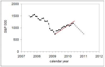
Because of the observed linear growth in N3 one can replace it with linear trends for the period between 2008 and 2011, as Figure 2 shows. This model predicts that the S&P 500 stock market index will be gradually decreasing at an average rate of 37 points per month. All fluctuations in N3, as observed in Figure 1, are smoothed in this linear representation.

Figure 1. Observed and predicted S&P 500 returns. The last point for the observed series is October 31, 2010.

Figure 2. The observed monthly closing level of the S&P 500 stock market index and the trend predicted from the number of nine-year-olds. The slope is of -37 points per month. The same but positive slope was observed between February 2009 and April 2010. The last point in the observed series is October 31, 2010. The deviation between the predicted and observed curves has been increasing since September 2010.

1987, 2001, 2008 … 2011

The essence of any quantitative model consists in the accuracy of prediction or predictive power. The higher is signal/noise ratio in a given data set the better can be the estimate of model parameters or the uncertainty of corresponding prediction. For the S&P 500 stock market index, the most prominent signals were measured during the periods of the fastest change: 1987, 2001 and 2008.

We have developed a model [1] linking the S&P 500 and its returns to the population of some characteristic age. The original model links the S&P 500 annual returns, Rp(t), to the number of nine-year-olds, N9:

Rp(t) = AdlnN9(t) + B (1)

where Rp(t) is the S&P 500 yearly return, A and B are empirical coefficients to be determined by some fitting procedure. They may change depending on the approximation used to represent N9. In the previous post on the S&P 500 returns we have approximated N9 by the number of three-year-olds, N3, six years before. Accordingly, we have obtained a prediction of the S&P return at a six year horizon, i.e. in 2010 one can foresee the returns in 2016. Relevant empirical relationship is as follows”

Rp(t+6) = 100dlnN3(t) - 0.23 (2)

Figure 1 depicts the S&P 500 returns, both actual one and that predicted by relationship (2). Both curves are coinciding in practical terms between 2008 and the middle of 2010.

In 1987 and 2001 abrupt falls in the returns were also observed. In this respect, the model also demonstrates an excellent predictive power, as Figures 2 and 3 depict. There are obvious differences between the measured S&P 500 returns. In 1987, the fall was very fast but not deep, from +0.3 to -0.1. In 2001, the returns declined gradually from +0.3 to -0.3 in 2002. In 2008, the observed curve fell from 0 to -0.5, i.e. approximately same as in 1987.

In all cases the model gives a good prediction of the timing and amplitude of the observed returns. So, the model has a good predictive power, considering that the prediction can be obtained at a nine year horizon with the birth rate used as a proxy to N9.

Therefore, one might treat our prediction of the 2011 fall as a reliable one.

During the last two weeks, the S&P 500 has been growing at a healthy pace. Currently, it exceeds the predicted level by approximately 50 to 100 points. This is a good reason to suggest that a significant force, which must eventually return the index to the trend line, has been developing in September 2010. If the growth continues into the second half of September one might expect a dramatic drop in October 2010. However, this will be just a part of the overall decrease to the level of -0.5 expected in July-August 2011.

Figure 1. The prediction of the S&P 500 annual return for the period between 2008 and 2012. We tentatively put the September's closing level at 1030.

Figure 2. The prediction of the S&P 500 annual return for the period between 1985 and 1989.

Figure 3. The prediction of the S&P 500 annual return for the period between 1998 and 2003.

References

1. Kitov, I., Kitov, O. (2010). S&P 500 returns revisited, http://ideas.repec.org/p/pra/mprapa/21733.html.

S&P 500 in September 2010

Good news from August 2010 is that the S&P 500 market index is back on the track predicted couple years ago. Figures 1 and 2 update the previous versions published on Seeking Alpha in August with the closing level of ~1050 reported on August 31. Both predicted curves are very close to the observed ones over the whole period between March 2009 and August 2010. This prediction would have been a convincing one for everybody except market players who do believe that stock prices are unpredictable.

So, we will continue tracking the level of S&P 500 and its returns. The next move is likely below the trend to compensate for a short positive excursion in July 2010. This might be a drop by 40 to 80 points, likely to the level below 1000. It might be accompanied by a small panic. However, a positive jerk associated with local positive news is not excluded but it should not be high in amplitude.

Our concern about possible repetition of the 1987 fall, if the index would continue its deviation from the predicted trend into October 2010, has been resolved by the drop of around 50 points from the July’s level of 1101. So, there is no danger of a severe panic on the stock market.

Below we repeat a mandatory part with a bit of mathematics for the readers interested in details of our excellent (in terms of predictive power) model. The model is also presented in our working paper [1] and monograph [2].

The original model links the S&P 500 annual returns, Rp(t), to the number of nine-year-olds, N9. In order to extend the prediction in time we use the number of three-year-olds, N3, as a proxy to N9 and obtain a forecast at a six-year horizon:

Rp(t+6) = 100dlnN3(t) - 0.23 (1)

where Rp(t+6) is the S&P 500 return six years ahead (in 2010 one can foresee the returns in 2016). Figure 1 depicts germane S&P 500 returns, both actual one and that predicted by relationship (1). Both curves are coinciding in practical terms.

Because of the observed linear growth in N3 one can replace it with linear trends for the period between 2008 and 2011, as Figure 2 shows. This model predicts that the S&P 500 stock market index will be gradually decreasing at an average rate of 37 points per month. All fluctuations in N3, as observed in Figure 1, are smoothed in this linear representation.

Figure 1. Observed and predicted S&P 500 returns. The last point for the observed series is August 2010.

Figure 2. Observed S&P 500 monthly close level and the trend predicted from the number of nine-year-olds. The slope is of -37 points per month. The same but positive slope was observed between February 2009 and April 2010. The last point in the observed series is August 2010. All in all, the S&P 500 is back on the predicted trend.

S&P 500 in August 2010

We continue tracking the evolution of the S&P 500 and our prediction made in the beginning of 2009 for the next six years. Since March 2009, the prediction fits the observed S&P 500 with minor deviations likely related to the emotion component of the stock market. However, the trend and its turn in May 2010 were forecasted precisely. All in all, fifteen months in a raw we are right and do not see any source which may disturb our prediction for the period between June 2010 and 2014. The prediction was documented in a working paper (S&P 500 returns revisited) and several posts.

The original model links the S&P 500 annual returns, Rp(t), to the number of nine-year-olds, N9. To obtain a prediction we use the number of three-year-olds, N3, as a proxy to N9 at a six-year horizon:

Rp(t+6) = 100dlnN3(t) - 0.23 (1)

where Rp(t+6)is the S&P 500 return at a six-year horizon. Figure 1 depicts relevant S&P 500 returns, both actual one and that predicted by relationship (1). The former curve has been approaching the latter one since May 2010.

Because of the linearity in the N3 growth one can replace it with linear trends for the period between 2008 and 2011, as Figure 2 shows. This model predicts that the S&P 500 stock market index will be gradually decreasing at an average rate of 37 points per month. All fluctuations in N3, as observed in Figure 1, are smoothed in this linear representation.

In July, actual closing level was ~1100 (+50 relative to June 2010). As predicted in the post devoted to the July’s level of S&P 500, the panic behavior observed in May and June 2010 ended in July (the quiet period continues into August 2010). However, we expected the close level between 1020 and 1050 in July 2010. Actual level was 50 points above the expected one, which is the effect of dynamic overshoot.

Figure 2 shows that the level of S&P 500 was above the trend line in July 2010. In the first decade of August 2010, the level of S&P 500 has been hovering around 1100. It may stay at this level by the end of August. In this case the difference between the actual and trend levels will be growing. If this tendency will stretch into September 2010, the difference will increase above 100 points. This will create a potential, which may express itself in a force returning the S&P 500 to the trend level with likely overshoot well below the trend. Same effect was observed in 1987. The cumulated potential may release in a market crash, if the level of S&P 500 will not be decreasing in August and September 2010. So, it will be interesting to follow up the future S&P 500 trajectory.

Figure 1. Observed and predicted S&P 500 returns.

Figure 2. Observed S&P 500 monthly close level and the trend predicted from the number of nine-year-olds. The slope is of -37 points per month. The same but positive slope was observed between February 2009 and April 2010.

S&P 500 in July 2010

We continue tracking the evolution of the S&P 500 and our prediction made in the beginning of 2009 for the next six years. Since March 2009, the prediction fits the observed S&P 500 with minor deviations likely related to the emotion component of the stock market. However, the trend and its turn in May 2010 were forecasted precisely. All in all, fifteen months in a row we are right and do not see any source which may disturb our prediction for the period between June 2010 and 2014. The prediction was documented in a working paper (S&P 500 returns revisited) and several posts .

The original model links the S&P 500 annual returns, R_p(t), to the number of nine-year-olds, N₉. To obtain a prediction we use the number of three-year-olds, N₃, as a proxy to N₉ at a six-year horizon:

R_p(t+6) = 100dlnN₃(t) - 0.23

where R_p(t+6)is the S&P 500 return at a six-year horizon. Because of the properties of the N₃ distribution one can replace it with linear trends for the period between 2008 and 2011, as Figure 1 shows. The model shown in Figure 1 predicts that the S&P 500 stock market index will be gradually decreasing at an average rate of 37 points per month. (Correction from the previous post where 46 points per months was used by mistake.) In June, actual closing level was 1030 (-60 relative to May 2010). This level is about 90 points below that predicted in Figure 1. This is the continuation of the May’s panic. Such dynamic "overshoot" in the beginning of a new trend is a common feature.

Figure 1. Observed S&P 500 monthly close level and the trend predicted from the number of nine-year-olds. The slope is of -37 points per month. The same but positive slope was observed between February 2009 and April 2010.

The deviation from the new trend is a big one and one can expect the end of panic in July/August 2010. This is a nice feature of the trend. Any deviation, whatever amplitude it has, must return to the trend. So, by the past experience we may judge that 90 points should be compensated quickly. This means that the level of S&P 500 should not change much in July and August 2010. We would expect the close level between 1020 and 1050 in July 2010.

Then, the index will continue gradual decrease into 2011. Figure 2 demonstrates that the S&P 500 annual return will sink below zero in the third-fourth quarter of 2010.

Figure 2. Observed and predicted S&P 500 returns.

S&P 500 in June 2010

As has already been discussed many times since March 2009 and also documeted in a working paper (S&P 500 returns revisited), we expect the S&P 500 stock market index to be gradually decreasing at an avearge rate of 46 points per month. In this post on S&P 500 (01/05/2010), we put the closing level of S&P 500 in May 2010 at 1132 (miscalculation, should be 1142). The actual closing level was 1090 (-97 relative to April 2010), i.e. 42 points below the predicted one. One could expect that kind dynamic "overshoot" in the beginning of a new trend. Same purely emotional effect was observed in March (+69) and April 2009 (+74), when the S&P 500 was increasing much faster than the average rate for the whole period of the rally between March 2009 and April 2010.

So, one might not exclude that the panic of May 2010 will last another month and the closing level of S&P 500 in June will be below 1095, as would be predicted by the rate of -46 points per month starting with 1187 in April 2010. By the end of the summer, the fall will likely decelerate. But the overall downward trend will continue and extend into 2011.

S&P 500 in May 2010

The fall in the S&P 500 index, predicted a year ago and well documented in a working paper (S&P 500 returns revisited) and a monograph, did happened in May 2010. On May 29, 2010, one more trade day on May 31, the level of S&P is around 1090. According to our model is should be 1132 by the end of May.

The yearly returns started to fall in April-May because the growth in April 2010 was smaller that than in April 2009. Figure 1 demonstrates relevant monthly returns. May 2010 is the first month since March 2009 when S&P sinks below the previous month’s level.

Figure 2 compares the S&P 500 returns with those predicted from real GDP reading. Lately, the BEA has revised its estimate for 2010Q1 down to 3.0% from the previous estimate of 3.2%. We included the revision into the predicted curve. Figure 3 displays the most recent period to show the start of the fall. So, the fall has starter, and likely will extend into 2011. In terms of GDP, there should be not more than 5% in 2010Q2. According to the fall in S&P 500, the second half of 2010 will be characterized by low growth rate.

Figure 4 depicts the model linking S&P 500 to the number of 9-year-old, N9. The future numbers of N9 are represented by the number of 3-year-olds, N3, shifted six years ahead. All in all, the level of S&P 500 should suffer a further fall into 2011.

We will be reporting the comparison of the observed and predicted S&P 500 in due course.

Figure 1. Monthly S&P 500 returns

Figure 2. Observed yearly S&P 500 returns and those predicted from real GDP according to the relationship shown in the low left corner of the panel.

Figure 3. Same as in Figure 2 since January 2009.

Figure 4. Observed yearly S&P 500 returns and those predicted from the number of 3-year-olds (at a six year horizon). The relationship is presented in the Figure. In June, the S&P 500 index show fall by another 46 points.

CXO and S&P 500 returns

I appreciate the reader's interest to our recent paper "S&P 500 returns revisited" , which resulted in the review made by CXO experts. I have no specific comments on the review except mainly qualitative charater of the assessment. The paper is chiefly quantitative, however.

In this sense, no words can justify our statements, only observations. A year ago, we predicted the fall in May 2010. See what will happen next, and lets revisit the CXO assessment in December 2010. If the model is wrong - everybody will see that it is wrong.

S&P 500: decline and fall

A year ago we predicted a kink in the growth of S&P 500 returns in April-May 2010. This prediction is accurate enough with S&P 500 increased with lower increment in April and May 2010 than it was in April and May 2009.

We've just published a paper (S&P 500 returns revisited) on the prediction where we have put the S&P 500 closing level in April 2010 at 1187 (actual was 1186.68). In May 2010, the (monthly closing) index should fall to 1132 and manifest the start of absolute decrease. So, what we have been recently observing was a decline and we will observed the fall, likely extended into 2011.

Relevant data:
stock prices - finance.yahoo
real GDP - Bureau of Economic Analysis
population - Census Bureau

Figure 1. Observed and predicted S&P 500 returns (12-month cumulated). Notice the turn from growth to fall in April-May 2010. The predicted returns are obtained from the model linking S&P 500 to real GDP. See details in the paper cited in the text.

Figure 2. Observed and predicted S&P 500. Red line was predicted in March 2009. The turn in May 2010 is expected with S&P 500 falling from 1187 to 1132. The model links S&P 500 and the number of 9-year-olds, as presented in the paper. According to our estimates, the absolute level of the index may sink below 1000 before 2011 and even 200-250 deeper by July 2011. As before, we display several figures with absolute S&P 500 and its returns.

Figure 3. The prediction of the S&P 500 returns between May 2010 and December 2011. The (12-month cumulated) returns will drop to -0.5. At monthly rates, the returns will be around -0.05 in December 2010.

One may find it interesting to compare our predictions to those made at POLITICAL CALCULATIONS, the only independent blog we have a link to.

S&P 500 returns revisited

working paper has been published by MPRA:

S&P 500 returns revisited

Ivan O. Kitov, Oleg I. Kitov

Abstract

The predictions of the S&P 500 returns made in 2007 have been tested and the underlying models amended. The period between 2003 and 2008 should be described by the dependence of the S&P 500 stock market index on real GDP because the population pyramid was highly inaccurate. The 2008 trough and 2009 rally are well predicted by the original model, however. The rally will end in March/April 2010 and the S&P 500 level will be decreasing into 2011. This prediction should validate the model.

Key words: S&P 500, returns, prediction, population pyramid, GDP

JEL Classification: G1, D4, J1

The probability to get rich

Another monograph has been published and is available on amazon.com
Mechanics of personal income distribution. The probability to get rich

The processes behind distribution of personal incomes and related measures of inequality have always been in the center of political and economic discussions. We have developed a microeconomic model which accurately describes the shape of personal income distribution (PID), as estimated in the Current Population Surveys. The model predicts the age-dependent PIDs as a function of real economic growth and demography. The underlying physical concept was borrowed from geo-mechanics. Our approach serves as a firm basis for definitions of income inequality. Officials, both government and financial, might be interested in the projections of poverty levels and mean incomes. For economists, the model provides a new tool of quantitative research. For the broader scientific community, the model links economics to hard sciences. All readers may estimate the probability to get rich depending on age and current income.

The S&P 500 returns will drop to -0.05 in 2011

Believe you or not, we predicted the fall in the S&P 500 returns in March 2009. In February 2009, there was no indication of the following linear growth in the returns. Below we present our model and predictions for 2010 and 2011. The model in best described in (Kitov, 2010).

The returns will drop again to -0.5!

S&P 500 returns and real GDP
As discussed in (Kitov, Kitov and Dolinskaya, 2009), there exists a trade-off between the growth rate of real GDP pre capita and the change rate of the number of 9-year-olds. Corresponding relationship should work in both directions and the number of 9-year-olds can be estimated from GDP measurements. So, one can replace N9(t) with GDPpc(t), taking into account that second term in the relationship between real GDP per capita and population is constant.
Figure 1 displays the observed S&P 500 returns and those obtained using real GDP, as presented by the US Bureau of Economic Analysis (http://www.bea.gov/). The observed returns are presented by MA(12) of the monthly returns. The predicted returns, Rp(t), are obtained from the following relationship:

Rp(t) = 0.6*dln(GDPpc(t)) - 0.0092,

where GDPpc(t) is represented by MA(6) of the (annualized) growth rate during or six previous months or two quarters as only quarterly readings of real GDP are available.
The period after 1996 is relatively well predicted including the increase in 2003. Therefore, it is reasonable to assume that the 9-year-old population was not well estimated by the US Census Bureau after 2003. This conclusion is supported by the cointegration test conducted for real GDP per capita and the charge rate of the number of 9-year-olds, which proves the existence of a long-term equilibrium linear relation between these two variables since the early 1960s (Kitov, Kitov and Dolinskaya, 2009). As a result, one can use either N9(t) or GDPpc(t) for modeling of the S&P 500 returns, where appropriate. Obviously, the GDPpc(t) is consistent with the S&P 500 returns after 2003.

Figure 1. The observed and predicted S&P 500 returns. The latter are obtained using quarterly readings of the growth rate of real GDP. One may expect rapid economic growth in 2010.

There is a concern related to the accuracy of population and real GDP measurement in 2006. In Figure 1, the predicted curve fell to -0.075 in the third quarter of 2006. There was no significant decrease in the S&P 500 returns during the same period. A possible reason for the discrepancy is that the real GDP was underestimated. This issue should be resolved in the next comprehensive revision to the GDP.
A striking feature in Figure 1 is the agreement between the annual curves in 2008 and 2009. The GDP readings predict the S&P 500 returns in time and amplitude. Moreover, the S&P index leads the GDP curve and predicts a rapid real economic growth in 2010. This is a good prediction to validate the link. All in all, real GDP per capita is a good predictor of the S&P 500 returns, especially during periods of big changes.

Using the number of 3-year-olds and the model linking it to the S&P 500 returns we have predicted the evolution between 2008 and 2014. The graph shown in Figure 2 is borrowed from (Kitov, 2010) with the amendments related to 2010.

If the level of S&P 500 will not reach 1200 by the end of March 2010, it will manifest the start of the fall. In any case, April 2010 will be the last months with growth, if any. Since May 2010, the fall is inevitable. It will be fast and deep – down to -0.5 (cumulative over the previous 12 months) by August 2011. One should bear in mind, that all predictions for 2009 and the beginning of 2010 have been realized.

Figure 2. Observed and predicted S&P 500 returns. By August 2011, the 12-month cumulative return will drop to -0.5. The period between March 2009 and March 2010 was predicted with high accuracy, taking into account the change in calibration.

Figure 3. The S&P 500 returns are currently reaching the peak with the following fall down to -0.04 (in average over the previous 12 months) by August 2011, as Figure 2 shows.

KITOV, I. KITOV, O., DOLINSKAYA, S. (2009). Modelling Real Gdp Per Capita In The Usa:Cointegration Tests, Journal of Applied Economic Sciences, Spiru Haret University, Faculty of Financial Management and Accounting Craiova, vol. 4(1(7)_ Spr)

Kitov, I. (2010). Deterministic mechanics of pricing. Saarbrucken, Germany, LAP Lambert Academic Publishing.

PREDICTING REAL ECONOMIC GROWTH IN FRANCE, GERMANY, NEW ZEALAND, AND THE UNITED KINGDOM

Journal of Applied Economic Sciences (JAES) has published the spring issue with my paper:

Ivan O. KITOV, 2010. "Predicting Real Economic Growth In France, Germany, New Zealand, And The United Kingdom," Journal of Applied Economic Sciences, Spiru Haret University, Faculty of Financial Management and Accounting Craiova, vol. 5(1(11)_Spr), pages 48-54.


Abstract
The growth rate of real GDP per capita is modeled and predicted at various time horizons for France, Germany, New Zealand, and the United Kingdom. The rate of growth is represented by a sum of two components – a gradually decreasing trend and fluctuations related to the change in country-specific age population. The trend is an inverse function of real GDP per capita with constant numerator. Previously, similar models were developed and validated for the USA and Japan.

Keywords: real GDP per capita, modeling, prediction, population

JEL classification: E1, E3, O4, O5

Dramatic decline in labor force participation

Michael Mandel at “Economics Unbound” is really interested in labor force participation rate (LFPR). He devoted couple previous posts to related problems in an attempt to explain the evolution of labor force participation rate and productivity by some modern and fancy reasons. It is not worth to repeat his posts here and I just refer to Figure 1 as a general argument against any short-term force driving LFPR. The overall trajectory has a very clear picture of secular oscillations. Between 1965 and 2000, the LFPR was growing with just minor plateaus near 1980m and 1990. After 2000, the LFPR has been declining. This is a robust downward trend which hardly to be compensated by innovations, as Michael suggests.

In 2009, the LFPR has decreased from 66% to 65.4% in Q3 with average over the three quarters of 65.6%. A 0.6% drop in LFPR is a dramatic one. It corresponds to ~2,000,000 people leaving labor force in the US almost at once! (It is worth noting that such a drop may severely affect the rate of unemployment because people without job are more likely to leave labor force). According to our model [1], this the decline in the LFPR was expected in 2010. However, the population estimates, which are used for the prediction, have never been accurate enough for sharp timing. In any case, the model developed in [1-3], which links LFPR and productivity in developed countries to real GDP per capita has proved its consistency. The next two to three years should serve for further validation, as Figure 2 assumes.

Figure 1. The evolution of LFPR between 1960 and 2009.

Figure 2. The observed LFPR and that predicted from real GDP per capita. We expect the LFPR to fall down to 64.5% by 2013.


The observed increase in productivity is directly related to the decrease in the LFPR. As a consequence, it was also well predicted by our model in [2]. We used the projection of the number of 9-year-olds from the number of 1-year-olds for the prediction of real GDP per capita in the 2010s. Since 2010, the productivity has to be growing, as Figure 5 in [2], demonstrates.

a)

b)

Figure 5. Prediction of the number of 9-year-olds by extrapolation of population estimates for younger ages (1- and 6-year-olds).
a) Total population estimates. The time series for younger ages are shifted ahead by 8 and 3 years, respectively.
b) Change rate of the population estimates, which is proportional to the growth rate of real GDP per capita. Notice the difference in the change rate provided by 1-year-olds and 6-year-olds for the period between 2003 and 2010. This discrepancy is related to the age-dependent difference in population revisions.
A downward trend in productivity, as has been observed since 2003, will turn to an upward one in the 2010s. This also means an elevated growth rate of real GDP per capita during the period between 2010 and 2017.


References

[1] Kitov, I., Kitov, O., (2008). The Driving Force of Labor Force Participation in Developed Countries, Journal of Applied Economic Sciences, Spiru Haret University, Faculty of Financial Management and Accounting Craiova, vol. III(3(5)_Fall), pp. 203-222. http://www.jaes.reprograph.ro/articles/3_TheDrivingForceofLaborForceParticipationinDevelopedCountries.pdf

[2] Kitov, I., Kitov, O., (2008). The driving force of labor productivity, MPRA Paper 9069, University Library of Munich, Germany, http://ideas.repec.org/p/pra/mprapa/9069.html
http://mpra.ub.uni-muenchen.de/9069/01/MPRA_paper_9069.pdf

[3] Kitov, I., Kitov, O., (2009). Modelling and predicting labor force productivity, MPRA Paper 15152, University Library of Munich, Germany, http://mpra.ub.uni-muenchen.de/15152/01/MPRA_paper_15152.pdf

Semi-annual report on SP 500: from April to September 2009

This is a semi-annual report on the evolution of S&P 500 index. It compares the actually observed monthly closing levels to those predicted by our model, as originally presented in [1]. The major conclusion is that the prediction of a monotonic growth in S&P level made in March 2009 is correct. There is no indication that the growth will end before May 2010, where we foreseen the turn to a negative slope. Accordingly, the S&P 500 annual return will soon reach positive figures and will be growing at an accelerated rate till May 2010.

The model links S&P 500 annual returns to the number of 9-year-olds and has passed econometric tests for cointegration, with goodness-of-fit reaching 0.9. Since the number of 9-year-olds can be accurately predicted using younger cohorts, one can predict S&P returns at a several-year horizon. (Standard demographic projections may be used to predict over a decade ahead.)

We revealed the link between S&P 500 and the number of 9-year-olds in December 2007 using historical data since 1985. Since the very beginning of 2008, we have been carefully tracking the evolution of S&P 500. The original model actually predicted a sharp fall in 2008 [1]. (As in many scientific studies, the attempt to improve the original model, in order to fit data between 2003 and 2007, had failed, as we reported in this blog at several occasions.) The re-calibrated version of the original model developed in March 2009 is as follows:

Rp(t) = 165dln[N3(t+6)] - 0.17 (1),

In (1), Rp is the 12-month cumulative return; N3 is the number of three-year-olds; t+6 – time shifted by six years ahead to extrapolate the number of 3-year-olds into the number of 9-year-olds; dln is the rate of growth, i.e. the monthly increment in N3 normalized to the contemporary level. The time step is one month or 1/12 of a year.

Figure 1 compares the initial prediction of the S&P 500 evolution, the observed trajectory for the period since February 2009, and a new prediction till 2011. Relationship (1) is used with the number of 9-year-olds extrapolated from the number of 3-year-olds. In March 2009, we used a preliminary calibration of the original model and assumed the monthly increment in S&P 500 would be 80 points. This assumption was too optimistic and the growth was weaker. The original prediction is shown by blue lin with solid circles in Figure 1, and the observed values are shown by red diamonds. The black line represents an updated prediction since September 2009. It reproduces the old prediction but with a 46-point monthly increment since October 2009, as discussed below.

All in all, Figure 1 presents strong evidence in favour of our original model. Six months of almost monotonic growth were not expected by many market players in March 2009. The next nine months should bring additional validation to the model. The most important event will be the turn in May 2010. But the growth before this date is of crucial importance as well.

Figure 1. The evolution of S&P 500. Blue line - the original prediction using (1) with 80 unit per month increment. Red line – observations. Black line – the updated prediction since October 2009 with a 46-point monthly increment.

In any case, the model predicts a sudden drop in 2008 and 2009 to the level of 700, which has been followed by constant growth to the level 1050 in September 20009. Initially, we estimated the peak value in 2010 as 1800. But the last six months demonstrated the necessity to re-calibrate the model using new data. (In physics, even fundamental constants are under permanent re-estimation, and empirical and even fundamental models are constantly recalibrated.) Therefore, we also re-estimated coefficients in (1) to fit the last six S&P 500 (monthly) readings. The new model is as follows:

Rp(t) = 135dln[N3(t+6)] - 0.17 (2),

Actually, we needed to reduce the coefficient of linear term from 165 to 135 with free term unchanged. Figure 2 depicts the updated prediction of the S&P 500 annual returns. The peak S&P 500 value in May 2010 should be 1425 (not 1800) if the future increment will be 46 points per month, as observed between March and September 2009.

Figure 2. Observed and predicted S&P 500 returns. The September level of S&P 500 index is 1057. The past six months are relatively well predicted.

Conclusion
Between 1985 and 2009, the S&P 500 returns can be accurately described by population estimates. The model based on the number of 9-year-olds produces a time series which is cointegrated with the S&P 500 returns, i.e. reveals a weak causality, as proved by the cointegration tests.

The re-calibrated model predicts the continuation of S&P 500 growth into 2010 with the peak level of ~1400 in May. The annual returns will reach positive zone soon and also peak in May 2010 at the level of 50% to 70%.


References
[1] Kitov, I., Kitov, O., (2007). Exact prediction of S&P 500 returns, MPRA Paper 6056, University Library of Munich, Germany, http://ideas.repec.org/p/pra/mprapa/6056.html

S&P 500 in July 2009

Stock market behavior has always been a source of surprises for researchers, traders, and investors. The long term aggregate price trends have been explained as related to fundamental factors. These factor, however, are numerous and not well defined. As a result, no prediction is possible.
In [1] we presented selected results of modelling, which demonstrate the robustness of long-term (years!) prediction. In the model, only one factor drives trends and fluctuations ain S&P 500. Therefore, our results are easy to interpret and repeat. Since March 2009, S&P 500 has been growing. This fast growth was foreseen in February 2009. Since March 2009, we have been reporting comparisons of monthly returns – observed and predicted. So far, the match is excellent.
In this post, preliminary results for July 2009 are reported, as accompanied by formal introduction of the model. The model is an empirical one and needs to be assessed and (sometimes) updated when new data are available. The last assessment (published in this blog) was carried out in June 2009. Since the model links S&P 500 to the growth rate in real GDP, we made relevant forecast for the second quarter of 2009 as +5%. This value is very high compared to the consensus (Conference Board) prediction of -0.7% .

1. S&P 500 vs. the number of nine-year-olds
To begin with, in Figure 1 we present observed and predicted S&P 500 returns for the period between 1985 and 2003 and their residual. Main finding is that the observed and predicted time series are cointegrated [1], both according to the Engle-Granger tests and the Johansen approach, i.e. there exists a long-term equilibrium relation between S&P 500 returns and the number of 9-year-olds in the USA. The latter is the driving force of the stock market and real GDP.

We have been carefully tracking the evolution of S&P 500 since 2007, when predicted a sharp fall in 2008 [1]. The updated relationship between S&P 500 returns and the (extrapolated) number of nine-year-olds is as follows:

Rp(t) = 165dln[N3(t+6)] - 0.17 (1),

In (1), Rp is the 12-month cumulative return; N3 is the number of three-year-olds; N9 is the number of 9-year-olds; t+6 – time shifted by six years ahead to extrapolate the number of 3-year-olds into the number of 9-year-olds.

Figure 2 predicts S&P 500 index using the number of 9-year-olds extrapolated from the number of 3-year-olds. There are two new points, June (919) and July (~990) 2009, since the last update in June 2009. The latter figure is a preliminary one as picked on July 30, 2009. It is not likely that this figure will change dramatically during the last trading day in July.
A sudden drop in 2008 and 2009 to the level of 700 should be followed by an increase to 1800 in 2010. Notice that the start of the current growth in S&P 500 was first predicted in March 2009, when the market was very low with the close at ~735 in February. The last five points together with the turn to the growth were forecasted.

Figure 2. Evolution of S&P 500. Red line – observations; black line – prediction from the number of 9-year-olds. The prediction is obtained using (1).

2. S&P 500 vs. real GDP per capitaThe main problem for an accurate prediction consists in the fact that the number of 9-year-olds in the end of any decade is prone to high bias. Only decennial censuses (next due in 2010) allow adequate estimates. Because of high uncertainty in N9, we have proposed to use real GDP per capita, GDPpc, as a proxy to the N9 [2-3]. Originally, the link between real GDP growth rate and the change rate of the number of 9-year-olds was found by Kitov [4]. Corresponding relationship should work in both directions, i.e. one can estimate the growth rate of real GDP from population measurements, and the number of 9-year-olds from real GDP measurements.

In relationship (1), we replace N9(t) with GDPpc(t), taking into account that second term in the relationship between real GDP per capita and population is constant. Figure 3 displays the observed S&P500 returns and those obtained using real GDP, as presented by the US Bureau of Economic Analysis (http://www.bea.gov/). As before, the observed returns are 12-month cumulative values. The predicted returns are obtained from the relationship

Rp(t) = 15.0*dln(GDPpc(t)) - 0.32 (2)

where GDPpc(t)) is represented by the average (annualized) growth rate during four previous quarters. It is worth noting that there are no monthly readings of real GDP available. Hence, only quarterly figures can be compared.

The period after 2000 is well predicted including the sharp increase in 2003. Therefore, it is reasonable to assume that the 9-year-old population was not well estimated by the US Census Bureau after 2003. This conclusion is supported by the cointegration test conducted for real GDP per capita and the charge rate of the number of 9-year-olds [3], which proves the existence of a long-term equilibrium linear relation between these two variables since the early 1960s. As a result, one can use either N9(t) or GDPpc(t) for the modelling of the S&P 500 returns, where one of them is more appropriate. Obviously, the GDPpc(t) is consistent with the S&P 500 returns after 2007. The years between 2007 and 2010 should confirm or reject this statement.
Currently, relationship (2) holds. The deep fall in 2008-2009 is well described. It also predicts that real GDP will start to increase in the nearest future following the observed increase in S&P 500. It would be very strong evidence in favour of (2).
Today the BEA will announce the Q2 figure. In Figure 3, red circle is our prediction (made a month ago) for 2009Q2. The rate of growth should be +5% relative to the previous quarter. The BEA should also provide a comprehensive revision to all historical reading of GDP. We expect a positive revision to real GDP estimates during the last four years.
In June, S&P 500 did not change from its May level of 919. (In May 2009, it grew by +47 units from 872 to 919). In July, the June non-growth is likely to be compensated with a rise by approximately 80 points from 919 to ~1000. Figure 4 shows the past and future predictions using the number of 3-year-olds.

Figure 3. The link between S&P 500 returns and real GDP per capita between 2000 and 2009. Red circle is a prediction of the growth rate for 2009Q2. The rate of growth is taken at the level of +5% relative to previous quarter.

Figure 4. Observed and predicted S&P 500 returns. The July level of S&P 500 index is around 1000, from its level of 919 in June 2009. The past five months are relatively well predicted.

ConclusionBetween 1985 and 2009, the S&P 500 returns can be accurately described by population estimates and readings of real GDP per capita. The model based on the number of 9-year-olds produces a time series which is cointegrated with the S&P 500 returns, i.e. reveals a weak causality, as proved by the cointegration tests. The next event to support the presence of the link between GDP and S&P 500 is the announcement of the growth rate in Q2 2009. From Figure 3, one can expect a positive figure, which is likely to be larger than 1 or 2 percentage points.


References[1] Kitov, I., Kitov, O., (2007). Exact prediction of S&P 500 returns, MPRA Paper 6056, University Library of Munich, Germany, http://ideas.repec.org/p/pra/mprapa/6056.html

[2] Kitov, I., Kitov, O., Dolinskaya, S., (2008). Comprehensive Macro – Model For The US Economy, Journal of Applied Economic Sciences, Spiru Haret University, Faculty of Financial Management and Accounting Craiova, vol. 3(4(6)_Wint), pp. 405-418. http://www.jaes.reprograph.ro/articles/winter2008/ComprehensiveArticle8.pdf

[3] Kitov, I., Kitov, O., Dolinskaya, S., (2009). Modelling real GDP per capita in the USA: cointegration tests, Journal of Applied Economic Sciences, Spiru Haret University,Faculty of Financial Management and Accounting Craiova, vol. 4(1(7)_ Spr), pp. 80-96. http://www.jaes.reprograph.ro/articles/spring2009/KitovI_KitovO_DolinskayaS.pdf

[4] Kitov, I., (2006). GDP growth rate and population, Working Papers 42, ECINEQ, Society for the Study of Economic Inequality, http://ideas.repec.org/p/inq/inqwps/ecineq2006-42.html

Cointegration tests of the model for real GDP growth

Originally, this article was published in the Journal of Applied Eeconomic Sciences:

Kitov, I., Kitov, O., Dolinskaya, S., (2009). Modelling real GDP per capita in the USA: cointegration tests, Journal of Applied Economic Sciences, Spiru Haret University,Faculty of Financial Management and Accounting Craiova, vol. 4(1(7)_ Spr), pp. 80-96.

We have already introduced at Seeking Alpha the model for the evolution of real GDP per capita in developed countries. Specifically we presented models for Japan [1], France, Germany, New Zealand, and the UK [2], and demonstrated that the model allows prediction of GDP at various time horizons. Originally the model was revealed using exceptional population estimates reported for the USA [3]. Moreover, we have conducted a cointegration test, which has confirmed the presents of a long-term equilibrium relation between real GDP per capita and the change in population of country-specific age. To begin with, we re-introduce the model.

Model and data

There is a measured macroeconomic variable characterized by a long-term predictability for a large developed economy. This is the annual increment of real GDP per capita. One can distinguish two principal sources of the intensive part of real economic growth, i.e. the evolution of real GDP per capita, G: the change in the number of 9-year-olds, and the economic growth trend associated with per capita GDP, G_t. The trend has the simplest form – no change in mean annual increment, as expressed by the following relationship:

dG_t(t)/dt = A (1)

where G(t) is the absolute level of real GDP per capita at time t, A is an empirical and country-specific constant. The solution of this ordinary differential equation is as follows:

G_t(t) = At + B (2)

where B=G_t(t₀), t₀ is the starting time of the studied period. Then, the relative growth rate (or economic growth trend) of real GDP per capita is:

g_trend(t) = dG_t/G_tdt = A/G (3)

which indicates that the (trend) rate is inversely proportional to the attained level of the real GDP per capita and the growth rate should asymptotically decay to zero.

One principal correction has to be applied to the per capita GDP values published by the Bureau of Economic Analysis. This is the correction for the difference between the total population and the population of 15 years of age and above. Our concept requires that only this economically active population should be considered when per capita values are calculated.

Following the general concept of the two principal sources of real economic growth one can write an equation for the growth rate of real GDP per capita, g_pc(t):

g_pc(t) = dG(t)/(dt‧G(t)) = 0.5dN₉(t)/(dt‧N₉(t)) + g_trend(t) (4)

where N₉(t) is the number of 9-year olds at time t. One can obtain a reversed relationship defining the evolution of the 9-year-old population as a function of real economic growth:

d(lnN₉(t)) = 2(g_pc - A/G(t))dt (5)

Equation (5) defines the evolution of the number of 9-year-olds as described by the growth rate of real GDP per capita. The start point of the evolution has to be characterized by some (actual) initial population. However, various population estimates (for example, post- and intercensal one) potentially require different initial values and coefficient A.

Instead of integrating (5) analytically, we use the annual readings of all the involved variables and rewrite (5) in a discrete form:

N₉(t+Δt) = N₉(t)[1 + 2Δt(g_pc(t) - A/G(t))] (6)

where Δt is the time unit equal to one year. Equation (6) uses a simple representation of time derivative of the population estimates, where the derivative is approximated by its estimate at point t. The time series g_pc and N₉ are independently measured variables. In order to obtain the best prediction of the N₉(t) by the trial-and-error method one has to vary coefficient A and (only slightly in the range of the uncertainty of population estimates) the initial value - N₉(t₀). The best-fit parameters can be obtained by some standard technique minimising the RMS difference between predicted and measured series. In this study, only visual fit between curves is used, with the average difference minimised to zero. This approach might not provide the lowermost standard deviation.

Equation (6) can be interpreted in the following way - the deviation between the observed growth rate of GDP per capita and that defined by the long-tern trend is completely defined by the change rate of the number of 9-year olds. A reversed statement is hardly to be correct - the number of people of some specific age can not be completely or even in large part defined by contemporary real economic growth. Specifically, the causality principle prohibits the present to influence the birth rate nine years ago. Econometrically speaking, the number of 9-year olds has to be a weakly exogenous variable relative to contemporary economic growth.

In fact, Eq. (6) provides an estimate of the number of 9-year-olds using only independent measurements of real GDP per capita. Therefore, the amplitude and statistical properties of the deviation between the measured and predicted number of 9-year olds can serve for the validation of (4) and (5).

Cointegration test

Skipping unit root tests we continue with a number of cointegration tests. The assumption that the measured number of 9-year-olds in the USA, N_9m(t), and that predicted from the real economic growth, N_9p(t), are two cointegrated non-stationary time series is equivalent to the assumption that their difference, e(t)=N_9m(t) - N_9p(t), is a stationary or I(0) process. The predicted and measured series corresponding to the post- and intercensal population estimates are shown in Figures 4 and 6, and their differences in Figures 5 and 7, respectively.

Figure 4. Comparison of the measured and predicted postcensal population estimates between 1960 and 2002.
Figure 5. The difference between the measured and predicted population estimates presented in Figure 4. For the period between 1962 and 2002, the average difference is 0 and standard deviation is 164926 for coefficient A=547.1325 and the initial value for the population of 3900000 in 1959. Linear regression is represented by a bold straight line.

Figure 6. Comparison of the measured and predicted intercensal population estimates between 1960 and 2002.

Figure 7. The difference between the measured and predicted population estimates presented in Figure 6. For the period between 1962 and 2002, the average difference is -1 and standard deviation is 165744 for coefficient A=546.079 and the initial value of population of 3900000 in 1959. Linear regression is represented by a bold straight line.

It is natural to start with unit root tests in the difference. If e(t) is a non-stationary variable having a unit root, the null hypothesis of the existence of a cointegrating relation can be rejected. Such a test is associated with the Engle-Granger approach, which requires the N_9m(t) to be regressed on the N_9p(t) as the first step, however. It is worth noting, that the predicted variable is obtained by a procedure similar to that of linear regression and provides the best visual fit between corresponding curves. The Engle-Granger approach is most reliable and effective when one of the two involved variables is weakly exogenous, i.e. is driven by some forces not associated with the second variable. This is the case for the GDP per capita and the number of 9-year-olds. The latter variable is hardly to be driven by the former one. The existence of an opposite causality direction is the main object of this study.

The results of the ADF and DF-GLS tests, listed in Table 3, demonstrate the absence of a unit root in the measured-predicted difference series for both the post- and intercensal population estimates. Since the predicted series are constructed in the assumption of a zero average difference, trend specification in these tests is “none”. The maximum lag order in the tests is 3. These results give strong evidences in favor of the existence of a cointegrating relation between the measured and predicted time series. Therefore, from the econometric point of view, it is difficult to deny that the number of 9-year-olds is the only defining force behind the observed fluctuations of the real economic growth. These fluctuations are observed around the growth trend defined by constant annual increment, A, of the real GDP per capita.

Table 3. Unit root tests for the differences between the measured and predicted number of 9-year-olds. Trend specification is constant. The maximum lag order is 3.

Test	Lag	Time series		1% critical
		postcensal	intercensal
ADF	0	-2.87*	-2.85*	-2.64
	1	-3.67*	-3.59*	-2.64
	2	-2.99*	-3.92*	-2.64
	3	-2.90*	-2.83*	-2.64
DF-GLS	1	-3.55*	-3.47*	-2.64
	2	-2.98*	-2.92*	-2.64
	3	-2.92*	-2.85*	-2.64

The next step is to use the Engle-Granger approach again and to study statistical properties of the residuals obtained from linear regressions of the measured and predicted single year of age populations. A pitfall of the regression analysis consists in a slight time shift between the measured and predicted series – the former variable is assigned to July 1 (averaged population) and the latter to December 31 (cumulative GDP increase) of the same year. Such a phase shift, apparently, results in a deterioration of regression results but can not be recovered since only annual population estimates are available before 1980.

Table 4 presents a summary of relevant unit root tests with the same specifications as accepted for the difference of the same series. The null hypothesis of a unit root presence is rejected for both time series and all time lags. Therefore, the residuals of the regression build an I(0) time series, and the Engle-Granger tests proves that the predicted and measured variables are cointegrated.

Table 4. Unit root tests for the residual time series of a linear regression of the measured series on the predicted one. The measured and predicted series are the numbers of 9-year-olds. Trend specification is none (zero average value of the residuals) and maximum lag order 3.

Test	Lag	Time series		1% critical
		postcensal	intercensal
ADF	0	-3.03*	-3.02*	-2.64
	1	-3.88*	-3.86*	-2.64
	2	-3.15*	-3.13*	-2.64
	3	-3.05*	-3.01*	-2.64
DF-GLS	1	-3.71*	-3.69*	-2.64
	2	-3.06*	-3.04*	-2.64
	3	-2.98*	-2.95*	-2.64

The Johansen approach is based on the maximum likelihood estimation procedure and tests for the number of cointegrating relations in the vector-autoregressive representation. The Johansen technique allows simultaneous testing for the existence of cointegrating relations and determining their number (rank). For two variables, only one cointegrating relation is possible. When cointegration rank is 0, any linear combination of the two variables is a non-stationary process. When the rank is 2, both variables have to be stationary. When the Johansen test results in rank 1, a cointegrating relation between the involved variables does exist.

In the Johansen approach, one has first to analyze some specific properties of the underlying VAR model for the two variables. Table 5 lists selection statistics for the pre-estimated maximum lag order in the VAR. Standard trace statistics is extended by several useful information criteria: the final prediction error, FPE; the Akaike information criterion, AIC; the Schwarz Bayesian information criterion – SBIC; and the Hannan and Quinn information criterion, HQIC. All tests and information criteria in Table 5 indicate the maximum pre-estimated lag order 1 for VARs and vector error-correction models, VECMs. Therefore, the maximum lag order 1 was used in the Johansen tests along with “constant” as the trend specification.

Table 5. Pre-estimation lag order selection statistics. All tests and information criteria indicate the maximum lag order 1 as an optimal one for VARs and VECMs.

	Lag	LR	FPE	AIC	HQIC	SBIC
postcensal	1	63.03*	5.8e+09*	25.31*	25.36*	25.44*
intercensal	1	61.63*	6.1e+09*	25.38*	25.42*	25.51*

FPE - the final prediction error, AIC - the Akaike information criterion, SBIC - the Schwarz Bayesian information criterion, HQIC - the Hannan and Quinn information criterion

The properties of the VAR error term have a critical importance for the Johansen test [8]. A number of diagnostic tests was carried out for the VAR residuals. The Lagrange multiplier test for the postcensal time series resulted in χ² of 0.34 and 0.09 for lags 1 and 2, respectively. This test accepts the null hypothesis of the absence of any autocorrelation at these lags. The Jarque-Bera test gives χ²=7.06 (Prob>0.03) with skewness=0.96 and kurtosis=3.77, the skewness being of the highest importance for the normality test and the validity of statistical inference. Hence, the residuals are probably not normally distributed, as expected from the artificial features of the measured population time series. The VAR model stability is guaranteed by the eigenvalues of the companion matrix, which are lower than 0.63. As a whole, the VAR model accurately describes the data and satisfies principal statistical requirements applied to the residuals.

Table 6 represents some results of the Johansen tests. In both cases the cointegrating rank is 1. Hence, there exists a long-run equilibrium relation between the measured and predicted number of 9-year-olds in the USA. The predicted number is obtained solely from the readings of real GDP per capita measured and reported by the BEA. We do not test for the causality direction between the variables because the only possible way of influence, if it exists, is absolutely obvious.

Table 6. Johansen test for cointegration rank for the measure and predicted time series. Trend specification is constant. Maximum lag order is 2.

Time series	Rank	Eigenvalue	SBIC	HQIC	Trace statistics	5% critical value
postcensal	1	0.397	52.48*	52.23*	2.198*	3.76
intercensal	1	0.379	52.55*	52.30*	2.117*	3.76

In this Section, three different tests have demonstrated at a high level of confidence that the measured and predicted number of 9-year-olds in the USA are cointegrated. One can use the cointegrating relation for a reliable prediction of real economic growth in the USA. This finding proves that the evolution of a developed economy is predictable in principle.

References

[1] Kitov, I., (2006). The Japanese economy, MPRA Paper 2737, University Library of Munich, Germany, http://ideas.repec.org/p/pra/mprapa/2737.html

[2] Kitov, I., (2009). Predicting real GDP per capita in France, Germany, New Zealand, and the UK, MPRA Paper 15503, University Library of Munich, Germany

[3] Kitov, I., (2006). GDP growth rate and population, Working Paper 42, ECINEQ, Society for the Study of Economic Inequality.