5/23/12
Time to buy SPY
8/13/11
Time to buy stocks
6/13/11
Angry Bear on the relation between S&P 500 and GDP
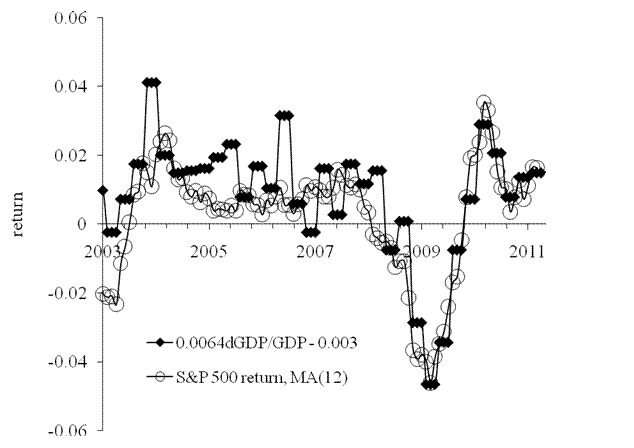
Actually, the S&P 500 returns are coitegrated with the change rate of real GDP per capita and this correlation is not spurious as shown in this blog and our paper on S&P 500.
6/5/11
Forecasting S&P 500 returns. Quarterly update
3/3/11
Modeling S&P 500 returns. March 2011
11/7/10
Black Tuesday?
This observation raises a question on the following events. Our concern about possible repetition of the 1987 fall, if the index would continue its deviation from the predicted trend into October 2010 is on again. So, I see a danger of a severe panic on the stock market. Because Tuesday is a common day for such events, I cannot exclude that one of Tuesdays in the nearest future will end in a return of the observed curves to the predicted one.
There is also a chance that the population estimates underlying the prediction become wrong since September 2010. The methods of population projection and updates used by the Census Bureau are also not well predicted.
Below we repeat a mandatory part with a bit of mathematics for the readers interested in details of our model. The model is also presented in our working paper [1] and monograph [2].
The original model links the S&P 500 annual returns, Rp(t), to the number of nine-year-olds, N9. In order to extend the prediction in time we use the number of three-year-olds, N3, as a proxy to N9 and obtain a forecast at a six-year horizon:
Rp(t+6) = 100dlnN3(t) - 0.23 (1)
where Rp(t+6)is the S&P 500 return six years ahead (in 2010 one can foresee the returns in 2016). Figure 1 depicts germane S&P 500 returns, both actual one and that predicted by relationship (1). Both curves are coinciding in practical terms.
Because of the observed linear growth in N3 one can replace it with linear trends for the period between 2008 and 2011, as Figure 2 shows. This model predicts that the S&P 500 stock market index will be gradually decreasing at an average rate of 37 points per month. All fluctuations in N3, as observed in Figure 1, are smoothed in this linear representation.
Figure 1. Observed and predicted S&P 500 returns. The last point for the observed series is October 31, 2010.
Figure 2. The observed monthly closing level of the S&P 500 stock market index and the trend predicted from the number of nine-year-olds. The slope is of -37 points per month. The same but positive slope was observed between February 2009 and April 2010. The last point in the observed series is October 31, 2010. The deviation between the predicted and observed curves has been increasing since September 2010.
9/14/10
1987, 2001, 2008 … 2011
9/1/10
S&P 500 in September 2010
8/19/10
S&P 500 in August 2010
7/29/10
Procter and Gamble on rise?
7/28/10
PepsiCo share price
IBM share price on decline
7/27/10
Xilinx share price
References
Kitov, I. (2010). Deterministic mechanics of pricing. Saarbrucken, Germany, LAP Lambert Academic Publishing.
Ball Corporation share price
Schlumberger share price
7/26/10
HPQ share price
So, the best-fit 2-C model for HPQ(t) is as follows:
HPG(t) = -3.20FB(t-4) +2.91RPR(t-5) + 3.64(t-2000) - 50.82
Figure 1. Evolution of the price of DAIRY and TPU.
Figure 2. Observed and predicted HPQ share prices. Original prediction is shown by red line. Black diamonds present the original line shifted 4 months ahead, i.e. the model.
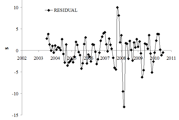
Figure 3. Residual error of the model. Mean residual error is 0 with standard deviation of $2.13. The largest errors were observed in 2007.
References
Kitov, I. (2010). Deterministic mechanics of pricing. Saarbrucken, Germany, LAP Lambert Academic Publishing.
MMM share price
So, the best-fit 2-C model for MMM(t) is as follows:
MMM(t) = -0.74DAIRY(t-10) – 0.54TPUP(t-6) + 8.70(t-2000) + 180.88
The model does predict the share price in the past and foresee a significant fall in the last quarter of 2010, i.e. through December 2010. It will be in line with the overall fall in the S&P 500 in 2010.
Figure 1. Evolution of the price of DAIRY and TPU.
Figure 2. Observed and predicted MMM share prices. Original prediction is shown by red line. Black diamonds present the original line shifted 6 months ahead.
Figure 3. Residual error of the model. Mean residual error is 0 with standard deviation of $3.79. The largest errors were observed in 2005 and 2006.
References
Kitov, I. (2010). Deterministic mechanics of pricing. Saarbrucken, Germany, LAP Lambert Academic Publishing.
7/25/10
Predicting DeVry's share price
According to [1], the model for DeVry (DV) is defined by the index for the rent of primary residency (RPR-CUUS0000SEHA) and that of pets, pet products and services (PETS-CUUR0000SERB). The former CPI component leads the share price by 11 months and the latter one leads by 4 months. Figure 1 depicts the overall evolution of both involved indices. From our past experience, the larger is the lag the more unreliable is the model. However, both defining components provide the best fit model between August 2009 and June 2010. The positive influence of RPR (+7.90) is compensated by the negative input of all other terms . So, the best-fit 2-C model for DV(t) is as follows:
DV(t) =7 .90RPR(t-11) – 2.76PETS(t-4) - 35.73(t-2000) - 757.63
The predicted curve in Figure 2 leads the observed price by 4 months with the residual error of $3.24 for the period between July 2003 and June
The model does predict the share price in the past and foresees A significant fall in the next quarter, i.e. through September 2010. It will be in line with the overall fall in the S&P 500 in 2010.

Figure 1. Evolution of the price of RPR and PETS.

Figure 2. Observed and predicted DV share prices . Original predcition is shown by red line. Black diamonds present the original prediction shifted by 4 months ahead.
Prediction of Legg Mason share price
According to [1], the model for Legg Mason (LM) is defined by the index of food (F-CUUS0000SAF ) and that of appliances (APL-CUUR0000SEHK). The former CPI component leads the share price by 4 months and the latter one leads by 13 months. From our past experience, the larger is the lag the more unreliable is the model. However, both defining components provide the best fit model between August 2009 and June 2010. Both coefficients in the LM model are positive. This means that increasing food price forces the share price up. The fall in the index of appliances has been compensating *see Figure 1) both the increase in F and positive linear time trend in the share price, as defined by the slope of +33.024. So, the best-fit 2-C model for LM(t) is as follows:
LM(t) =
The predicted curve in Figure 2 leads the observed price by 4 months with the residual error of $6.89 for the period between July 2003 and June
The model does predict the share price in the past and foresees no significant increase in the next quarter, in July through September 2010. Considering the overall fall in the S&P 500 in 2010, one should not expect any growth in stock prices at all.
Figure 1. Evolution of the price index of food (F) and appliances (APL).The latter has been falling since July 2009.
Figure 2. Observed and predicted LM share prices.
Figure 3. Residual error of the model. Mean residual error is 0 with standard deviation of $6.89. the largest errors were observed in 2005 and 2006.
References
Kitov,
Drang nach Osten — «натиск на Восток»
ИИ гугла написал « Drang nach Osten — «натиск на Восток») — это исторический термин, обозначающий германскую экспансию на славянские и восто...
-
These are two biggest parts of the Former Soviet Union. To characterize them from the economic point of view we borrow data from the Tot...
-
These days sanctions and retaliation is a hot topic. The first round is over and we will likely observe escalation well supported by po...
-
Yesterday I missed the absolute hero of deflation in the US – the consumer price index of information technology, hardware and software (see...