Revisiting JNJ share price

Recently, the BLS has reported the CPI estimates for March 2011. It is natural to revisit our models for the first quarter. Johnson & Johnson (JNJ) is one of the companies we have been following since 2009. A preliminary model was obtained in September 2009. The latest model was reported in January 2011.  

Originally, the stock price was defined by the index of appliances (APL) and that of transportation services (TS). We have revisited the stock in September 2010 and found that the model did not change, except a slight change in coefficients well explained by the uncertainty of the monthly closing price as a parameter characterizing the stock behavior and the estimation accuracy of these two defining CPIs.

In the previous post on JNJ we presented a model based on the CPIs for November 2010 and the December closing price of JNJ. Our concept of share pricing and quantitative approach is described in [1]. Briefly, we decompose a share price into a weighted sum of two individual CPI components and minimize the RMS model error.

Figure 1 depicts the overall evolution of both involved consumer price indices. These two defining components provide the best fit model between March 2009 and March 2011, i.e. two years or 24 months.  Since the index of appliances has been on a steady decline since the early 2000s, its negative coefficient of -1.35 (-1.40 in January) has actually resulted in the growth of the share price. The negative influence of TS, -1.47 (-1.26), has been also compensated by all other terms in the model.  The best-fit 2-C model for JNJ(t) is as follows:

JNJ(t) = -1.35APL(t-2) – 1.47TS(t-6) + 11.13(t-1990) + 332.20

Actually, the predicted curve in Figure 2 leads the observed price by 2 months with the residual error of $2.35 (see Figure 3) for the period between March 2003 and March 2011. One may conclude that the price of a JNJ share is well defined by the behaviour of the two defining CPI components.

Comparing the evolution of the observed and predicted prices since the start of modelling (2008) we have found that the model does predict the share price in the past and foresees at a two month horizon.

In January, we expected that this share would experience a slight growth in the first quarter of 2011. The price actually has stalled at the level of $60. In the second quarter 2011, the price should not change much.

Figure 1. Evolution of the price of APL and TS.

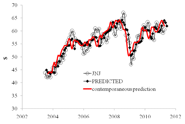
Figure 2. Observed and predicted JNJ share prices. Red line – contemporaneous prediction which forecasts major pivot points in advance.

Figure 3. Residual error of the model. Mean residual error is 0 with standard deviation of $2.35. The largest errors were observed in 2007 and 2010.  Currently, the model overestimates the share price.

References

Kitov, I. (2010). Deterministic mechanics of pricing. Saarbrucken, Germany, LAP Lambert Academic Publishing.

BSX in Q1 and Q2

The price model for Boston Scientific (BSX) was reported in January 2011, as based on our stock pricing concept [1]. We expected a small rise in the price in 2011Q1.  The original model included the consumer price index of housing (H) and the index of durable goods (DUR). The former defining CPI component led the share price by 5 month and the latter one by 3 months. The updated model has the same defining components and time lags. Figure 1 depicts the overall evolution of the involved indices.

These two defining components provide the best fit model between March 2011 and January 2010.  Both coefficients are negative, and thus the increasing prices result in decreasing share price. The slope of time trend is negligible. The best-fit 2-C model for BSX(t) is as follows:

 BSX(t) = -1.41H(t-5) – 2.85DUR(t-3) – 0.09(t-1990) + 630.92     

 where t is calendar time.  Both models predicted the price at a three month horizon with standard deviation of $1.83 between July 2003 and March 2011. There was no growth during  the first quarter of  2011 since no one of the defining indices has demonstarted any big movement. In the second quarter of 2011, the price may drop to the level of $5 from the current $7, as follows from the predicted and observed curves presented in Figure 2.

Figure 1. The evolution of H and DUR.

Figure 2. Observed and predicted BSX share prices. Red curve represents the contemporaneous prediction.

Figure 3. The model residual, i.e. the difference between the observed and predicted BSX share prices.

1. Kitov, I. (2010). Modelling share prices of banks and bankrupts, Theoretical and Practical Research in Economic Fields, ASERS, vol. I(1(1)_Summer) pp. 59-85

Why inflation will be low in 2011

Three months ago we reported that the price index of housing had been decreasing since the end of 2008 relative to the overall CPI. This is a sustainable negative trend in a CPI subcategory with the highest input in the overall CPI. The housing index comprises approximately a half of the headline CPI.

Figure 1 displays the difference between the CPI and the housing index (both not seasonally adjusted) as reported by the BLS on April 14, 2011. The current trend is positive (the CPI grows faster than the index of housing) and the difference has been growing at a rate of +0.4 per month. Between 1996 and 2007, the slope was -0.06 per month.

FBR’s Vice Chair Yellen discussed the evolution of commodity and consumer prices over the past year and found that

… Turning now to the outlook for U.S. consumer prices, I anticipate that the recent surge in commodity prices will cause headline inflation to remain elevated over the next few months. However, I expect that consumer inflation will subsequently revert to an underlying trend that remains subdued, so long as increases in commodity prices moderate and longer run inflation expectations remain reasonably well-anchored …

This statement does not contradict the long term trend in Figure 1. In several months, the current surge in energy prices will die and they likely return to the level of 2010. Then one will see a very low price inflation rate for 2011, as we predicted in 2005.

The decrease in the housing index (relative to the CPI)  will be accompanied by an effective stop in the food price growth and the fall in the transportation index relative to the CPI. All these effects will bring an extended period of deflation into the U.S. economy in 2012.

Figure 1. The change in the trend started in 2009. The current trend is positive (the CPI grows faster than the index of housing) and the difference has been growing at a rate of +0.4 per month. Between 1996 and 2007, the slope is -0.06 per month.

HPQ share price in 2011Q2

In the beginning of 2011, we revisited the share price model for HPQ and predicted no change for the period between the end of November ($42.1) and the closing price of the first quarter of 2011. Actually, the closing price was $40.26. There was a sharp peak in December 2010 ($45.69), however.

This time we use the CPI estimates published by the BLS on March 14. The newly obtained model is the practically same as before. It is defined by the index of food without beverages (FB) and that of rent of primary residency (RPR). Again, the former CPI component leads the share price by 4 months and the latter one leads by 5 months (i.e. one can predict at a four-month horizon). Figure 1 depicts the overall evolution of both involved indices. Considering the previous findings, these two defining components provide the best fit model between November 2009 and March 2010. One coefficient is negative and one is positive and the best-fit 2-C model for HPQ(t) is as follows:

HPQ(t) = -3.34F(t-4) + 3.41RPR(t-5) + 0.51(t-1990) – 85.44

This model is just slightly different from that estimated in January. The index of food has replaced that of food less beverages (FB). The difference between these indices is practically negligible, however. Both coefficients are practically the same as before. The predicted curve in Figure 2 leads the observed price by 4 months with the residual error of $2.29 for the period between July 2003 and March 2011.

The residual of the model in Figure 3 has demonstrated a quick recovery into the positive zone since the previous post.

For the second quarter of 2011, the model predicts the share price to fall to the level of $37 in June 2011 and even to $33 by the end of July 2011. Such a decrease will be a good validation for the model.

Figure 1. Evolution of the price of FB and RPR.

Figure 2. Observed and predicted HPQ share prices. The contemporaneous prediction is shown by red line. Black diamonds present the original line shifted 4 months ahead, i.e. the model. We expect the price to fall down to $33 in July 2011.

Figure 3. Residual error of the model.

Pepsico in 2011Q2

We have been studying the link between share prices and CPIs since 2008 [1]. The model for Pepsico (PEP) has been stable over the past year and is defined by the consumer price index of food at home (FH), which is a part of the food index, and the index information technology, hardware and software (IT). Both defining CPI components lead the share price by 4 and 8 months, respectively. Figure 1 depicts the overall evolution of the difference between the involved indices. There is a significant change in the trend in 2008 which potentially might cause a change in the sign of defining coefficients.

However, these two defining components provide the best fit model between March 2011 and July 2010.  Both coefficients are negative, and thus the increasing price indices result in a decreasing price of the share. The slope of time trend is positive revealing the price tendency to increase over time. The best-fit 2-C model for PEP(t) is as follows:

PEP(t) =  -1.51FH(t-4)  - 8.19IT(t-8)  + 2.47(t-1990)  + 414.78
    

where t is calendar time.

The predicted and observed curves are presented in Figure 2 and their difference in Figure 3. The residual error is of $2.28 for the period between June 2003 and March 2011. The model provides and an excellent and very stable prediction of the share price in the past and forecasts a significant fall in the price in the second quarter of 2011. It will be a larger challenge to the model. It is worth revisiting the PEP model in July 2011.

Figure 1. Evolution of the difference between FH and IT.

Figure 2. Observed and predicted PEP share prices.

Figure 3. The model residual, i.e. the difference between the observed and predicted PEP share prices.

1. Kitov, I. (2010). Modelling share prices of banks and bankrupts, Theoretical and Practical Research in Economic Fields, ASERS, vol. I(1(1)_Summer) pp. 59-85

Modeling share price for Boeing

We have been following the price of Boeing (BA) shares since early 2008. The original crude model included only major price indices, and specifically, the core CPI and the index of transportation. Then we extended the set of modeling indices to 92 and estimated an advanced model [1], which was not published, however. Since the model has been stable and accurate we have decided to present it.

 The model for Boeing has been stable over the past year and is defined by the consumer price index of furniture and bedding (FAB), which is a part of the housing index, and the index of pets, pet products and services (PETS). Both defining CPI components lead the share price by 1 month. Figure 1 depicts the overall evolution of the difference between the involved indices. There is no bigger change in the trend since 2003.

These two defining components provide the best fit model between March 2011 and July 2010.  The FAB coefficient is a positive one, and thus the increasing price of furniture and bedding leads to an increase in the share price one month later. The PETS index has a negative coefficient and causes the share price to fall. The slope of time trend is positive revealing the price tendency to increase over time. The best-fit 2-C model for BA(t) is as follows:

BA(t) =  3.47FAB(t-1)  - 5.96PETS(t-1)  + 42.20(t-1990)  –  298.50

where t is calendar time.

The predicted and observed curves are presented in Figure 2. The residual error is of $4.31 for the period between June 2003 and March 2011. The model provides and an excellent and very stable prediction of the share price in the past.

Figure 1. Evolution of the difference between FAB and PETS.

Figure 2. Observed and predicted BA share prices.

Figure 3. The model residual, i.e. the difference between the observed and predicted BA share prices.

 References

1. Kitov, I. (2010). Modelling share prices of banks and bankrupts, Theoretical and Practical Research in Economic Fields, ASERS, vol. I(1(1)_Summer) pp. 59-85

IBM share price in 2011Q1. Prediction for 2011 and 2012

Following the post on ADSK, we revisit our prediction of IBM share prices made in January 2011.  We also repeat the previous post on IBM in Appendix A in order to present our concept of share pricing and refresh the prediction. Overall we expected a healthy growth of the IBM share in 2011 and 2012 because the underlying model was very stable over the previous year and the trend in the difference between two defining CPI components (the consumer price index of motor vehicle insurance, MVI, and the index of housing, H) had not been changing since 1994.

The Bureau of Labor Statistics published new CPI estimates on 14.04.2011 and we have recalculated the model at the end of the first quarter.  The obtained model does not differ much from the previous one:

IBM(t) =  -4.60H(t-1) – 1.41MVI(t)  + 41.58(t-1990) + 803.15

 Both coefficients are practically the same, the time trend is slightly higher and the intercept is also by $24 higher. The lags are just one month shorter than in the previous model. Considering noisy data and the uncertainty in the (adjusted) monthly closing price, the original model is extremely stable.

The closing price in November 2010 was $146.76 and December 2010 - $162. The model predicted the price to grow to $142.4 by the end of March 2011. Actually, the price was $166.21. The increasing deviation may end up in a downward correction in Q2 or Q3 as it happened in July 2008 (see Figure 1). However, the overall growth in 2011 and 2012 should not be compromised by this correction, as discussed in Appendix A. We expect the share to rise.

Figure 1. The observed and predicted IBM share price in 2011Q1 and their difference.

Appendix A

Here we extend the modeling period in both directions - between January 1995 and December 2010.  As before, the model coefficients are obtained by minimizing the RMS residual error. Current IBM model is as follows:

IBM(t) =  -4.32*H(t-1) – 1.48*MVI(t-1)  + 40.69(t-2000) + 779.0

 where H is the index of housing and MVI  is the index of motor vehicle insurance. Figure 1 depicts the overall evolution of both involved indices. The index of housing was on rise before 2009. Since December 2008, this index has been slightly decreasing. Since it has negative influences on the share price, one can expect an increase in IBM price. The MVI index has been quickly growing over the entire period, except during some short segments.  Thus, did not allow the share to increase to fast since linear trend also has positive influence on the price.  All in all, these two defining components provide the best fit model between December 2009 and December 2010. 

The predicted curve in Figure 2 leads the observed price by 1 month with the residual error of $9.49 for the period between January 1995 and December 2010.  Currently, the price is slightly underestimated, as Figure 3 shows, and one cannot exclude a downward correction in the first quarter of 2011.

In the long run, the index of housing will be decreasing during the next 10 years. This is a helpful background for IBM share. The MVI has a clear rise/plateau structure. The next segment is likely to be a shelf, starting in 2011 of 2012. Hence, the price share looks good at a two-year horizon. 

Figure 1. Evolution of the price of H and MVI.

Figure 2. Observed and predicted IBM share prices.