Did we predict the new linear trend in the price index for "restaurants"?

A year ago, in response to the WSJ “Real Time Economics” post “Restaurant Prices to Flow Into ‘Core’ Inflation Measure” we evaluated the behavior of the price index for “full service meals and drinks” relative to the core CPI. Following our standard approach to small components of the CPI [1, 2], we calculated the difference between the core CPI and the index for “full service ..”. Figure 1 displays the difference as of June 2009.
As with many other components of the headline CPI [2], this difference is characterized by a linear trend between 1998 (start time of the index) and July 2008 with a slope +1.82. It means that the core CPI has been growing at a higher rate than the studied index during the past 10 years.

Since July 2008, a negative trend has been observed. Our naive assumption about this new trend was that it would repeat the previous one but with an opposite sign. Green line in Figure 1 represented the expected trend.

Figure 1. The difference between the core CPI and the price index for “full service meals and drinks”. Green line represents the expected trend between 2009 and 2018.

In 2011, we revisit this prediction and plot new data in Figure 2. As expected, the difference has reached the new trend line and slightly overshot it. In 2011, one cannot exclude the difference to decline below the new trend. Thus, the index of “restaurants” will be growing faster that the core CPI.

Figure 2. The difference has reached the new trend and slightly overshot the line. In 2010, one can expect the index of “restaurants” to grow faster than the core CPI.

References
[1] Kitov, I., Kitov, O., (2008). Long-Term Linear Trends In Consumer Price Indices, Journal of Applied Economic Sciences, vol. 3(2(4)_Summ), pp. 101-112, Spiru Haret University, Faculty of Financial Management and Accounting Craiova.
[2] Kitov, I., (2009). Apples and oranges: relative growth rate of consumer price indices, MPRA Paper 13587, University Library of Munich, Germany, http://mpra.ub.uni-muenchen.de/13587/01/MPRA_paper_13587.pdf

Cumulative inflation in Japan: 1982-2009

As promised in one of the previous posts, we present here a more detailed analysis of price inflation in Japan. The case of Japan is the best illustration of our inflation vs. labor force concept. Here we carry out an estimation of the empirical relationship between the change rate of labour force, dLF(t)/LF(t), inflation, pi(t).

Data on labour force and inflation were obtained from various sources. The Statistics Bureau of the Ministry of Internal Affairs and Communications provides information on various economic and demographic variables. The U.S. Bureau of Labour Statistics provides two sets of data: one obtained according to the national definition (NAC) and another obtained according to the U.S. definition of corresponding variable.

There are several measures for inflation. Most popular definitions for the overall price change are GDP deflator and Consumer Price Index. In many countries, the CPI definition was extended recently by imputed rent. Thus, various inflation time series might be studied, but only two of them are used. Figure 1 shows two inflation estimates: the OECD GDP deflator and the CPI provided by the Japanese Statistical Bureau. The difference between these curves is minor but very illustrative. The GDP deflator curve is consistently below CPI inflation since 1990.

Figure 1. CPI and GDP deflator in Japan.

As for many economic parameters, labour force estimates are also agency dependent due to various definitions and different population adjustments. Figure 2 compares the change rate of labour force provided by the OECD, Eurostat, according to national and U.S. definition. Despite strong similarity, discrepancies reaching 0.1 (or 10% of the total labour force) are observed. Such a difference is an important indicator of the difficulties in defining labour force. Further investigations are necessary to elaborate a consistent understanding of the term “labour force”. The model linking labour force change and inflation is likely a good candidate for quantitative consolidation of various definitions and approaches.

Figure 2. Comparison of four versions of the change rate of labour force in Japan: Eurostat, OECD, national accounts (NAC) and US definition.

First, we test the existence of a link between inflation and labour force. Because of the structural (measurement related?) break in the 1980s, we have chosen the period after 1982 for linear regression. By varying the lag between the labour force and inflation one can obtain the best-fit coefficients for the prediction of CPI inflation, pi(t), according to the following relationship:

pi(t) = 1.31dLF(t-t0)/LF(t-t0) + 0.0007 (1)

where the time lag t0=0 years; standard errors for both coefficients are shown in brackets. Figure 3 depicts this best-fit case. There is no time lag between the inflation series and the labor force change series in Japan. Free term in (1), defining the level of price inflation in the absence of labour force change, is practically undistinguishable from zero.

A more precise and reliable method to compare observed and predicted inflation consists in the comparison of cumulative curves. Short-term oscillations and uncorrelated noise in data as induced by inaccurate measurements and the inevitable bias in all definitions should be smoothed out in cumulative curves. Any actual deviation between two cumulative curves persists in time if measured values are not matched by the defining relationship. The predicted cumulative values are very sensitive to free term in (1). Therefore, in the upper panel of Figure 3 we use the slope obtained by the matching of cumulative curves shown in the lower panel of Figure 3:

pi(t) = 1.43dLF(t)/LF(t) + 0.000 (1′)

For Japan, the cumulative curves are characterized by complex shapes. There are periods of intensive inflation growth and a deflationary period. The labour force change, defining the predicted inflation curve, follows all the turns in the measured cumulative inflation. One can conclude that relationship (1) is valid and the labour force change is the driving force of inflation.

For obvious reasons, it is difficult to precisely estimate the change in labour force level during one year. However, there are some benchmark years when all previous estimates are revised in order to match a better measured level of labour force. So, one can expect an increasing relative precision of the change in labour force with increasing time baseline; the net change during 10 years should be measured with lower relative uncertainty than during one year.

Figure 3. Measured inflation (CPI) and that predicted from the change rate of labour force. Upper panel: Annual curves. Lower panel: Cumulative curves between 1982 and 2009. A good agreement between the cumulative curves illustrates the predictive power of our model.

Using relationships (1′), it is possible to quantitatively predict the evolution of inflation and unemployment through 2050 using various labour force projections. The National Institute of Population and Social Security Research provide quantitative projections of the total population, which can be used to obtain future estimates of the labour force. We consider the case of constant labour force participation rate fixed to 0.521, as measured in 2000. For this scenario, Figure 4 demonstrates that the level of labour force in Japan will decrease from 67,000,000 in 2010 to 57,000,000 in 2050.

Figure 4. Projection of the labour force evolution between 2005 and 2050.

Figure 5 displays the prediction of inflation until 2050. According to this prediction, 2009 was the last year of positive inflation (CPI) as Japan enters a prolonged deflationary period. The rate of depopulation will be accelerating after 2020. This will result in the increasing deflation approaching 1% per year on average. According to (1′), the overall population decline of 10 per cent will reduce the overall price level (CPI or GDP deflator) in Japan by approximately 15% by 2050. However, this forecast is based on an assumption about constant rate of labour force participation, which may also change over the next 40 years. Ageing population usually has lower participation rate.

Figure 5. CPI inflation rate in Japan through 2050.

One can conclude that the change rate of labour force is definitely the determining process behind inflation in Japan.

CHK, COP, CVX, DVN, ESV, HAL, and XOM. Improved models

Two days ago we revisited share price models for five energy companies from the S&P 500 list: ConocoPhillips (COP), Chevron (CVX), Devon Energy Corporation (DVN), Halliburton (HAL), and Exxon Mobil (XOM). Our pricing model links shares and CPI components (Kitov, 2009). It was demonstrated that all five original models, as had been obtained in 2008, predicted the time history of these prices with a good accuracy. In addition, since the difference between core CPI and headline CPI in the United States is well approximated by a linear function of time this difference can be used to predict share prices in the energy subcategory of the S&P 500 at time horizons of several years.

In this post we are going to improve these models for energy companies using an extended set of 17 individual CPIs, which includes all major subcategories of the headline CPI:

C headline CPI

F food and beverages

H housing

A apparel

T transportation

M medical care

R recreation

ED education

CO communication

O other goods and services

CE CPI less energy

CF CPI less food

CC core CPI

COMM commodities

E energy

NDUR nondurables

CFSHE CPI less food, shelter and energy

This step is in line with our general approach to price modeling, as described by Kitov (2010). We also introduce a quantitative measured of the prediction accuracy – RMSE (root-mean-square error) and check the predictive power of the underlying model.

The pricing model is common for all companies. We assume the presence of a linear link between a share price and the difference between the core (or headline) CPI and some other subset of goods and services comprising the headline CPI. The intuition behind the model is simple; a higher pricing power for a given subcategory of goods and services, and thus related companies, is expressed in a faster increase in corresponding stock prices. In the first approximation, the deviation between relevant price indices is proportional to the ratio of the pricing powers.

The pricing model states that a share price, SP(t), can be approximated by a linear function of the difference between two CPI components, dCPI:

SP(t) = A + B1CPI1(t + t1) + B2CPI2(t + t2) + C(t-t0) (1)

where A, Bi, and C are empirical constants for the studied period (between July 2003 (t0) and November 2010); t is the elapsed time; t1 and t2 are the time delays between the share and the CPIs, both to be determined. Here we introduce a linear trend element, C(t-t0), which has to compensate the trend component in the CPI difference (Kitov&Kitov, 2008). Without loss of generality we minimize the model error by standard LSQ method to find all 6 coefficients (A,Bi,C,ti) for those 2 CPI components among the set of 17, which provide the lowermost RMSE.

Figures 1 and 2 compare two updated predictions for COP and XOM obtained in the previous post with new model based on 17 components. The new models are as follows:

COP(t)= 2.69*H(t+8) – 0.76*T(t+1) – 12.47(t-2000) – 422.1; RMSE=$3.34;

XOM(t)= -2.44*F(t-12) - 1.13*O(t-13) + 31.84(t-2000) + 350.1; RMSE=$4.41

Figure 1. Upper panel: original observed and predicted COP price. A2=72, B2=-5.5 (1999-2009). Lower panel: the improved model described above. The prediction lags by 7 months behind the price.

Figure 2. Same as in Figure 1 for XOM. Original model is characterized by A2=90, B2=-6 (1999-2009).

Figures 3 through 5 compare the original and improved predictions for Chevron, Devon Energy, and Halliburton:

CVX = -5.5*(cCPI - CPI) +85; 1999-2009

CVX(t)= 3.16*H(t) – 10.51*R(t) – 0.90(t-2000) – 565; RMSE=$4.90;

DVN = -7.7*(cCPI - CPI) +97; 1999-2009

DVN(t)= 2.15*CF(t+1) – 0.50*E(t) – 9.72(t-2000) – 304.8; RMSE=$5.88;

HAL = -3.5*(cCPI - CPI) + 43; 1999-2009

HAL(t)= 0.40*T(t+1) – 0.90*O(t+6) + 11.64(t-2000) + 44; RMSE=$2.44

Figure 3. The original and improved share price prediction for CVX

Figure 4. The original and improved share price prediction for DVN

Figure 5. The original and improved share price prediction for HAL

All in all, the extension of the CPI set has significantly improved the predictive power of the model. We have also calculated models for other energy companies. Figure 6 displays two of them:

CHK(t)= -1.47*ED(t-7) + 0.41*E(t+1) +11.4(t-2000) – 12.1; RMSE=$2.68;

ESV(t)= 2.94*C(t) – 2.41*F(t-5) + 2.17(t-2000) – 113; RMSE=$4.14;

Figure 6. Models for CHK and ESV.

References

Kitov, I. (2009). ConocoPhillips and Exxon Mobil stock price, Journal of Applied Research in Finance, v. 2, pp. 129-134.

Kitov, I. (2010). Modelling Share Prices of Banks and Bankrupts, Theoretical and Practical Research in Economic Fields, Association for Sustainable Education, Research and Science, vol. 0(1), pages 59-85, June

Kitov, I., Kitov, O. (2008). Long-Term Linear Trends In Consumer Price Indices, Journal of Applied Economic Sciences, Spiru Haret University, Faculty of Financial Management and Accounting Craiova, vol. 3(2(4)_Summ), pp. 101-112.

Predicting shares of ConocoPhillips, Chevron, Devon Energy Corporation, Halliburton, and Exxon Mobil. 2010 revision

Approximately two years ago we introduced a concept linking share prices and CPI components (Kitov, 2009). To begin with, we modelled and predicted the evolution of share prices of ConocoPhillips (COP) and Exxon Mobil (XOM), which are classified in the S&P 500 list as related to energy. It was demonstrated that the time history of these prices could be accurately approximated by a linear function of the difference between core CPI and headline CPI in the United States. This difference is found to be the best to predict share prices in the energy subcategory of the S&P 500.

In this posts we are going to revisit those energy companies which shares were modelled in (Kitov, 2009) and (Kitov&Kitov, 2009) and check the predictive power of the underlying model. These companies are as follows: ConocoPhillips (COP), Chevron (CVX), Devon Energy Corporation (DVN), Halliburton (HAL), and Exxon Mobil (XOM).

The pricing model is common for all companies. It is simple. We assume the presence of a linear link between a share price and the difference between the core (or headline) CPI and some other subset of goods and services comprising the headline CPI. The intuition behind the model is simple; a higher pricing power for a given subcategory of goods and services, and thus related companies, is expressed in a faster increase in corresponding stock prices. In the first approximation, the deviation between relevant price indices is proportional to the ratio of the pricing powers. The presence of sustainable (linear or nonlinear) trends in the differences, as found in (Kitov&Kitov, 2008) allows predicting the evolution of the differences, and thus the deviation between prices for corresponding goods and services. The share prices have to follow up.

So, there exist sustainable trends in the differences between various subcategories of consumer (and producer) price indices. We consider the sustainability as an equivalent to the possibility to describe such trends by simple functions of time. Figure 1 shows that the difference between the core CPI, cCPI, and the headline CPI, CPI, can be approximated by a simple time function:

dCPI(t) = a + bt (1)

where dCPI(t) is the difference, a and b are empirical constants, and t is the elapsed time. Between 1981 and 1999, the linear trend has a slope +0.67, and from 2002 to 2008 the slope is (-1.65). Hence, the “distance” between the core CPI and the headline CPI is a linear function of time, with a positive or negative slope b. It might be of fundamental importance that absolute value of the ratio of the slopes is inversely proportional to the ratio of durations: │0.67/(-1.65)│≈7/19. If such a trade-off actually exists, one can predict the duration of the next trend from its slope.

Figure 1. The difference between the core CPI and the headline CPI between 1980 and 2008. There are two distinct periods from 1981 to 1999 and from 2002 to 2008, where the growth in the difference can be accurately approximated by linear functions of time with slopes +0.67 and -1.65, respectively. Notice that absolute value of the ratio of slopes is inversely proportional to the ratio of durations: │0.67/(-1.65)│≈7/19. The lower panel shows the beginning of the new trend in the difference.

Then, the pricing model states that a share price, for example, that of ConocoPhillips, COP(t), can be approximated by a linear function of the difference between the core and headline CPI (Kitov, 2009):

COP(t) = A + BdCPI(t + t1) (2)

where A and B are empirical constants (for COP, A=72 and B=-5.5) for the period between 1998 and 2009); t is the elapsed time; and t1=1/6 year is the time delay between the share and the CPI changes, i.e. the CPI has a lag behind the share price.

Empirical constants in (2) have to be determined for all distinct periods with different trends. This implies the possibility of structural breaks in the link between share price and CPI as caused by the turns to new trends. For example, the set of long-term economic bounds between goods and services, comprising the CPI and defining the linear trend in the dCPI between 1981 and 1999, underwent a three-year-long transition to a new set. In turn, the new set defined the trend observed from 2002 to 2008. So, it is reasonable to assume that the sign of slope in (2) should change to an opposite one after the end of the current transition period.

Figures 2 and 3 compare the original and updated predictions for COP and XOM. Coeffcients in (2) are given in the Figure captions.

Figure 2. The observed and predicted COP price. A2=72, B2=-5.5 (1999-2009). Upper panel - original model of 2009. Lower panel - updated for 2009 and 2010.

Figure 3. Same as in Figure 2 for XOM. A2=90, B2=-6 (1999-2009).

Figures 4 through 6 compare the original and updated predictions for Chevron, Devon Energy, and Halliburton. As for other energy-related companies, the difference driving relevant share prices is likely that between the core and headline CPI. The models for CVX, DVN, and HAL share price are the same in both cases:

CVX = -5.5*(cCPI - CPI) +85; 1999-2009

DVN = -7.7*(cCPI - CPI) +97; 1999-2009

HAL = -3.5*(cCPI - CPI) + 43; 1999-2009

The next move in all three shares will be up in line with the increasing oil price (Kitov, 2009). In the long run, the dCPI will likely be growing. The increasing difference will have the same effect on the prices in the future as always before – share price grows at a rate proportional to the slope in the dCPI.

Three companies in Figures 4 through 6 are characterized by different coefficients B between 2000 and 2010: from -3.5 (HAL) to -7.7 (DVN). Previously, we determined the slopes for COP (-5.5) and XOM (-6.0). Now one can conclude that these five energy-related companies demonstrate different levels of effectiveness in converting of the dCPI into share price.

Figure 4. The original and updated share price prediction for CVX

Figure 5. The original and updated share price prediction for DVN

Figure 6. The original and updated share price prediction for HAL

All in all, our concept gave a good prediction two years ago. All models are sound. Despite its striking dissimilarity to the mainstream concepts, our pricing model is deeply rooted in economics as expressed in terms of common sense: a higher pricing power achieved by a given company should be converted into a faster growth in corresponding consumer price index. So, the link between these two measured variables is, effectively, a causal one. If the evolution of the difference between various components of the CPI would have been a random walk, the mainstream stock pricing models would be correct. However, the existence of sustainable trends in the differences makes these models obsolete, at least for some companies from the S&P 500 list.

References

Kitov, I., (2009). ConocoPhillips and Exxon Mobil stock price, Journal of Applied Research in Finance, v. 2, pp. 129-134.

Kitov, I., Kitov, O., (2008). Long-Term Linear Trends In Consumer Price Indices, Journal of Applied Economic Sciences, Spiru Haret University, Faculty of Financial Management and Accounting Craiova, vol. 3(2(4)_Summ), pp. 101-112.

Kitov, I., Kitov, O. (2009). Modelling of selected S&P 500 share prices, MPRA Paper 15862, University Library of Munich, Germany.

Predicting DeVry's share price. December 2010 revision

The model for DeVry (DV) was introduces in July 2010. Originally, the stock price was defined by the index for the rent of primary residency (RPR-CUUS0000SEHA) and that of pets, pet products and services (PETS-CUUR0000SERB). We have revisited the stock and found that the model has not changed, except the time lag of the second defining CPI has increased from 4 to 5 months. The former CPI (RPR) component again leads the share price by 11 months. All coefficients are essentially as in the original model.

Figure 1 depicts the overall evolution of both involved indices. From our past experience, the larger is the lag the more unreliable is the model. However, both defining components provide the best fit model between November 2009 and December 2010. The positive influence of RPR (+7.10) is compensated by the negative input of all other terms. So, the best-fit 2-C model for DV(t) is as follows:

DV(t) =7 .10RPR(t-11) – 2.43PETS(t-5) – 31.90(t-2000) – 686.06

The predicted curve in Figure 2 leads the observed price by 5 months with the residual error of $3.68 for the period between March 2003 and December 2010. In other words, the price of a DV share is completely defined by the behaviour of the two CPI components.

Comparing the evolution of the observed and predicted prices since the start of modelling (2008) we have found that the model does predict the share price in the past and foresees at a four to five month horizon. One may expect a significant fall in the first quarter of 2011.

Figure 1. Evolution of the price of RPR and PETS.

Figure 2. Observed and predicted DV share prices. A contemporary prediction is shown by red line. Black diamonds present the original line shifted 5 months ahead.

Figure 3. Residual error of the model. Mean residual error is 0 with standard deviation of $3.68. The largest errors were observed in 2007 and 2008.

HPQ share price. December 2010 revision

Half a year ago we presented a model of the evolution of HPQ share price. We decomposed it into two CPIs, linear time trend and constant. It’s good time to revisit the prediction and the model.

According to [1], the model for Hewlett-Packard (HPQ) is defined by the index of food and beverages (F) and that of rent of primary residency (RPR). The former CPI component leads the share price by 4 months and the latter one leads by 5 months (i.e. one can predict at a four-month horizon). Figure 1 depicts the overall evolution of both involved indices. These two defining components provide the best fit model between November 2009 and December 2010. One coefficients is negative and one is positive together with time trend, with slope of 1.34.

So, the best-fit 2-C model for HPQ(t) share price is as follows:

HPQ(t) = -3.45F(t-4) +3.38RPR(t-5) + 1.34(t-2000) – 69.3

This model is slightly different from that in the previous post on HPQ. The index of food has replaced that of food less beverages (FB). The difference between these indices is practically negligible, however. Both coefficients are practically the same as before. Hence, the model has not changed in practical terms.

The predicted curve in Figure 2 leads the observed price by 4 months with the residual error of $2.39 for the period between March 2003 and December 2010. One can consider the price of a HPQ share as completely defined by the behaviour of the two CPI components.

The model does predict the share price in the past and foresaw the fall in 2010 four months in advance. The HPQ price is not expected to change in the first quarter of 2011.

Figure 1. Evolution of the price of F and RPR.

Figure 2. Observed and predicted HPQ share prices. The contemporaneous prediction is shown by red line. Black diamonds present the original line shifted 4 months ahead, i.e. the model.

Figure 3. Residual error of the model. Mean residual error is 0 with standard deviation of $2.29. The largest error was observed in July 2010 (-$6.31).

References

1. Kitov, I. (2010). Deterministic mechanics of pricing. Saarbrucken, Germany, LAP Lambert Academic Publishing.

How well can we predict the cumulative inflation ten years ahead?

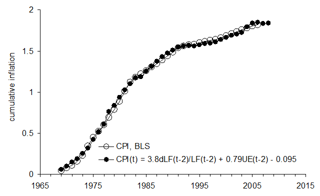
Our model of inflation [1] allows replacing price index with the cumulative growth of labor force. The biggest world developed economies all fit our model, as Figures 1 through 6 demonstrate (all borrowed from [1]). Moreover, the difference between observed and predicted cumulative inflation is a I(0) process, i.e. all observed/predicted pairs should be cointegrated. This allows linear regression, which is characterized by the goodness of fit above 0.99 for all presented cases: the USA, Austria, Canada, France, Germany, and Japan.

All observed curves have well predicted points of inflection. The most striking case is Japan, where the decline in labor force observed since the late 1990s manifests itself in deflation and cumulative curves (predicted and observed) have synchronized peak points.

We are going to consider each case in details, but it is crystal clear that the relative error of the proposed replacement (i.e. the prediction of cumulative inflation or price index) decreases with time and what one needs is a projection of labor force not all these forecasts of inflation. The former is usually is much more accurate than the latter.

Figure 1. USA

Figure 2. Austria

Figure 3. Canada

Figure 4. France

Figure 5. Germany

Figure 6. Japan