Modeling share prices: Morgan Stanley may continue growth

We built the first deterministic pricing model for Morgan Stanley (NYSE: MS) in November 2008 together with other companies from the S&P 500 list. Morgan Stanley was included in our study of bankruptcy cases in the USA [1]. The intuition behind our pricing concept was simple - a higher relative rate of price growth (fall) in a given subcategory of goods and services (as expressed by the consumer price indices – CPIs) is likely to result in a faster increase (decrease) in stock prices of related companies. In the first approximation, the deviation between price-defining indices is proportional to the ratio of their pricing powers.  The presence of sustainable (linear or nonlinear) trends in the differences between various CPIs allows predicting the evolution of these differences, and thus, the deviation between prices of corresponding goods and services. Such trends are the basis of a long-term prediction of share prices. In the short-run, deterministic forecasting is possible only when a given price lags behind the CPI components defining its behavior.

 

Why do we rely on consumer price indices in our modeling? Many readers may have reasonable doubts that any consumer price, which is not directly related to goods and services produced by a given company, may affect its price. We allow the economy to be a more complex system than described by a number of simple linear relations between share prices and goods. The connection between a firm and its products may be better expressed by goods and services which the company does not produce. The demand/supply balance is not well understood yet and may evolve along many nonlinear paths with positive and negative feedbacks. It would be too simplistic to directly define a company price by its products.

Overall, Morgan Stanley (MS) provides an example of a reliable pricing model. In [1] we reported that the defining CPIs in 2008 were the index of housing operations (HO) and the index of food away from home (SEFV). (For a short time in the second half of 2010, the defining indices were different: the index of food less beverages (FB) and the index of information technology, hardware and software (IT)). The model was revised in 2012 and the evolution of MS price was defined by the index of food away from home (SEFV) and owner’s equivalent rent of residence (ORPR), which is similar to HO. Hence, the model obtained in 2008 is the same as estimate in 2012. Figure 1 depicts the evolution of both indices. Here we revise the previous model with new data available for the period between November 2012 and March 2014. The defining indices, their coefficients and time lags are the same as in 2012. This observation validates the MS pricing model.

The best fit model, i.e. the lowermost RMS residual error, for February 2014 and October 2012 are as follows:  

 

MS(t) = -7.93SEFV(t-0) + 4.42ORPR(t-2) + 25.23(t-2000) + 420.92; October 2012

MS(t) = -7.57SEFV(t-0) + 4.26ORPR(t-2) + 23.66(t-2000) + 398.90; February 2014                

Table 1 lists the defining CPIs, model coefficients, lags, and standard errors for 15 models between March 2012 and February 2014. The predicted price curve in Figure 2 is in sync with the observed one. We also show the high and low monthly prices, which represent the uncertainty in the modeled price. One can use any price (e.g. high, low, mean, median) within a given month to model the overall evolution and obtain different coefficients and residuals. Therefore, the model for the losing price is a representative of a wider set of pricing models.

The model error for the period between July 2003 and February 2014 is $3.35.  The model accurately predicts the share price in the past. From the overall behaviour of the defining CPIs and the current negative residual (Figure 3) one may conclude that MS price is slightly underestimated, but the possible correction is within the uncertainty bounds. If the current trends in ORPR and SEFV are retained, MS may continue its growth.

 

Table 1. Defining CPIs, coefficients and standard errors of the models for 2012 and 2013/2014

 

Month	C1	t1	b1	C2	t2	b2	c	d	sterr,$
				2012
October	SEFV	0	-7.93	ORPR	2	4.415	25.226	420.919	3.468
September	SEFV	0	-7.90	ORPR	2	4.399	25.137	420.060	3.468
August	SEFV	0	-7.96	ORPR	2	4.425	25.343	423.817	3.447
July	SEFV	0	-7.96	ORPR	2	4.445	25.258	420.687	3.440
June	SEFV	0	-8.01	ORPR	2	4.449	25.526	426.655	3.437
May	SEFV	0	-8.01	ORPR	2	4.452	25.540	426.579	3.434
April	SEFV	0	-7.97	ORPR	2	4.419	25.492	427.246	3.422
March	SEFV	0	-8.00	ORPR	2	4.431	25.609	429.254	3.421
				2014	and	2013
February	SEFV	0	-7.569	ORPR	2	4.2574	23.66	398.90	3.35
January	SEFV	0	-7.605	ORPR	2	4.2773	23.81	400.40	3.33
December	SEFV	0	-7.735	ORPR	2	4.3249	24.43	411.33	3.28
November	SEFV	0	-7.732	ORPR	2	4.3197	24.44	411.77	3.29
October	SEFV	0	-7.740	ORPR	2	4.3231	24.47	412.41	3.30
September	SEFV	0	-7.754	ORPR	2	4.3227	24.57	414.62	3.31
August	SEFV	0	-7.810	ORPR	2	4.3494	24.80	418.21	3.32

 

 

 

 

 

 

 

 

 

 

 

 

Figure 1. Evolution of the price index of food away from home (SEFV) and owner’s equivalent rent of residence (ORPR). 

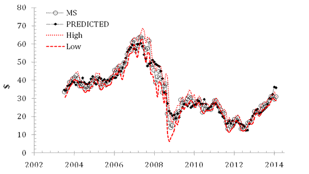
Figure 2. Observed and predicted MS share prices.

 

 

Figure 3. Residual error of the model. Mean residual error is 0 with standard deviation of $3.25.

 Appendix

In its general form, the pricing model is as follows:

sp(t_j) = Σb_i∙CPI_i(t_j-t_i) + c∙(t_j-2000 ) + d + e_j                                                                       (1) 

where sp(t_j) is the share price at discrete (calendar) times t_j, j=1,…,J; CPI_i(t_j-t_i) is the i-th component of the CPI with the time lag t_i, i=1,..,I; b_i, c and d  are empirical coefficients of the linear and constant term; e_j is the residual error, which statistical properties have to be scrutinized. By definition, the bets-fit model minimizes the RMS residual error. The time lags are expected because of the delay between the change in one price (stock or goods and services) and the reaction of related prices. It is a fundamental feature of the model that the lags in (1) may be both negative and positive. In this study, we limit the largest lag to fourteen months. Apparently, this is an artificial limitation and might be changed in a more elaborated model. In any case, a fourteen-month lag seems to be long enough for a price signal to pass through.

System (1) contains J equations for I+2 coefficients. Since the sustainable trends last more than five years, the share price time series have more than 60 points. For the current recent trend, the involved series are between 70 and 130 readings. Due to the negative effects of a larger set of defining CPI components their number for all models is (I=) 2. To resolve the system, we use standard methods of matrix inversion.

For the sake of completeness we always retain all principal subcategories of goods and services. Among them are the headline CPI (C), the core CPI, i.e. the headline CPI less food and energy (CC), the index of food and beverages (F), housing (H), apparel (A), transportation (T), medical care (M), recreation (R), education and communication (EC), and other goods and services (O). In this model, we use 92 CPI components. They are not seasonally adjusted indices and were retrieved from the database provided by the Bureau of Labor Statistics (2014).

There are two sources of uncertainty associated with the difference between observed and predicted prices. First, we have taken the monthly close prices (adjusted for splits and dividends) from a large number of recorded prices: monthly and daily open, close, high, and low prices, their combinations as well as averaged prices. Without loss of generality, one can randomly select for modeling purposes any of these prices for a given month. By chance, we have selected the closing price of the last working day for a given month. The larger is the fluctuation of a given stock price within and over the months the higher is the uncertainty associated with the monthly closing price as a representative of the stock price.

Second source of uncertainty is related to all kinds of measurement errors and intrinsic stochastic properties of the CPI. One should also bear in mind all uncertainties associated with the CPI definition based on a fixed basket of goods and services, which prices are tracked in few selected places.  Such measurement errors are directly mapped into the model residual errors. Both uncertainties, as related to stocks and CPI, also fluctuate from month to month.

Predicting share prices: Goldman Sachs Group may rise to $180-$200 per share in April

We have been trying to build a pricing model for Goldman Sachs Group (NYSE: GS) since 2008. This company was included in our study of bankruptcy cases in the USA. All in all, the model was not stable over time and the prediction for 2009 was not fully correct.  Originally, the stock price was defined by the index of housing operations (HO) and that of food away from home (SEFV).  In January 2011, we presented an updated model as based on the CPIs available till November 2010 and the December monthly closing (adjusted for splits and dividends) price of GS. In the updated model, the defining CPIs were the index of other food at home (OFH) and the housing index (H). Thus, the difference between the preliminary and the updated model was not too large because the pairs of defining indices are very close. In December 2012, we published a paper comparing GS with four financial companies and revised the model, which includes new data obtained since December 2010. Here we update the model using new data between December 2012 and March 2014. The 2012 model has not changed. This validates our approach to stock price modeling (see details in Appendix).

Table 1 lists defining parameters for GS between March and October 2012, and from August 2013 to February 2014. For each month, the best model is based on the same defining CPIs – the consumer price index of food and beverages, F, and the index of owners’ equivalent rent residence, ORPR.  In all cases, the lags are the same: three and two months, respectively. Other coefficients and the standard error suffer just slight oscillations or drifts (e.g. c and d). 

Figure 1 depicts the overall evolution of both involved consumer price indices: F and ORPR. The best-fit models for GS(t) are as follows:

GS(t) = -11.06OFH(t) +11.06H(t-12) - 1.82(t-2000) – 99.4, December 2010

GS(t) = -13.79F(t-3) +11.03ORPR(t-2) + 29.93(t-2000) + 33.75, October 2012

GS(t) = -13.038F(t-3) +10.556ORPR(t-2) + 30.44(t-2000) + 12.86, February 2014      

The predicted curve in Figure 2 leads the observed price by two months. The residual error is of $14.25 for the period between July 2003 and February 2014. The price of a GS share is relatively well defined by the behaviour of the two defining CPI components. Figure 2 also depicts the high and low monthly prices for the same period, which illustrate the intermonth variation of the share price. These prices might be considered as natural limits of the monthly price uncertainty associated with the quantitative model. Since 2009, the predicted price is well within the high/low band. Figure 3 displays the residual error. 

From Figure 2, the modeled price is approximately $200 in April 2014.

Table 1. The monthly models for GS for eight months in 2012 and for seven months in 2014/2013.

Month	C1	t1	b1	C2	t2	b2	c	d	sterr,$
				2012
October	F	3	-13.795	ORPR	2	11.027	29.935	33.751	14.521
September	F	3	-13.791	ORPR	2	11.013	29.992	35.827	14.584
August	F	3	-13.787	ORPR	2	11.003	30.023	37.106	14.649
July	F	3	-13.759	ORPR	2	10.978	30.018	37.647	14.707
June	F	3	-13.731	ORPR	2	10.933	30.124	41.985	14.758
May	F	3	-13.704	ORPR	2	10.876	30.342	48.755	14.770
April	F	3	-13.661	ORPR	2	10.819	30.449	53.171	14.805
March	F	3	-13.787	ORPR	2	10.943	30.440	48.639	15.055
				2014	and	2013
February	F	3	-13.038	ORPR	2	10.556	27.62	12.86	14.25
January	F	3	-13.3166	ORPR	2	10.660	28.88	34.69	14.02
December	F	3	-13.4606	ORPR	2	10.687	29.71	51.36	13.91
November	F	3	-13.4537	ORPR	2	10.676	29.75	52.34	13.96
October	F	3	-13.5352	ORPR	2	10.700	30.13	60.04	14.00
September	F	3	-13.5638	ORPR	2	10.683	30.44	67.71	14.03
August	F	3	-13.6031	ORPR	2	10.691	30.66	72.06	14.07

 

Figure 1. Evolution of F and ORPR.

 

Figure 2. Observed and predicted GS share prices. The prediction horizon is two months.

 

 

Figure 3. Model residuals, standard error of the model $14.25. 

 

Appendix

The concept of share pricing based on the link between consumer and stock prices has been under development since 2008. In the very beginning, we found a statistically reliable relationship between ConocoPhillips’ stock price and the difference between the core and headline consumer price index (CPI) in the United States. Then we extended the pool of defining CPIs to 92 and estimated quantitative models for all companies from the S&P 500. The extended model described the evolution of a share price as a weighted sum of two individual consumer price indices selected from this large set of CPIs. We allow only two defining CPIs, which may lead the modeled share price or lag behind it. The intuition behind the lags is that some companies are price setters and some are price takers. The former should influence the relevant CPIs, which include goods and services these companies produce. The latter lag behind the prices of goods and services they are associated with. In order to calibrate the model relative to the starting levels of the involved indices and to compensate sustainable time trends (some indices are subject to secular rise or fall) we introduced a linear time trend and constant term. In its general form, the pricing model is as follows:

sp(t_j) = Σb_i∙CPI_i(t_j-t_i) + c∙(t_j-2000 ) + d + e_j                         (1)                  

where sp(t_j) is the share price at discrete (calendar) times t_j, j=1,…,J; CPI_i(t_j-t_i) is the i-th component of the CPI with the time lag t_i, i=1,..,I (I=2 in all our models); b_i, c and d  are empirical coefficients of the linear and constant term; e_j is the residual error,  whose statistical properties have to be scrutinized.

By definition, the bets-fit model minimizes the RMS residual error. It is a fundamental feature of the model that the lags may be both negative and positive. In this study, we limit the largest lag to eleven months. System (1) contains J equations for I+2 coefficients. We start our model in July 2003 and the share price time series has more than 100 points. To resolve the system, standard methods of matrix inversion are used.  A model is considered as a reliable one when the defining CPIs are the same during the previous eight months. This number and the diversity of CPI subcategories are both crucial parameter.