The rate of unemployment on its way to 6% in December 2013

We have been reporting on the decline in the rate of unemployment in the US since the beginning of 2012. We predicted an extended unemployment fall period down to the level of 6.2% in the fourth quarter of 2013. This prediction was made after we accurately forecasted (on March 1, 2012) the rate of unemployment in the US to fall down to 7.8% by the end of 2012. Here we update our model and present the evolution of the unemployment rate in the second quarter of 2013. Overall, the measured rate has been following our prediction. We foresee the rate to fall down to 6% [±0.4%] in the fourth quarter of 2013 or in the first quarter of 2014.

In 2006, we developed three individual empirical relationships between the rate of unemployment, u(t), price inflation, p(t), and the change rate of labour force, LF(t), in the United States. We also revealed a general relationship balancing all three variables. Since measurement (including definition) errors in all three variables are independent it may so happen that they cancel each other (destructive interference) and the general relationship might have better statistical properties than the individual ones. For the USA, the best fit model for annual estimates was a follows:

u(t) = p(t-2.5) + 2.5dLF(t-5)/dtLF(t-5) + 0.0585   (1)

where inflation (CPI) leads unemployment by 2.5 years (30 months) and the change in labor force leads by 5 years (60 months). We have already posted on the performance of this model several times.

For the model in this post, we use monthly estimates of the headline CPI, u, and labor force, all reported by the US Bureau of Labor Statistics. The time lags are the same as in (1) but coefficients are different since we use month to month-a-year-ago rates of growth. We have also allowed for changing inflation coefficient. The best fit models for the period after 1978 are as follows:

u(t) = 0.63p(t-2.5) + 2.0dLF(t-5)/dtLF(t-5) + 0.07; between 1978 and 2003

u(t) = 0.90p(t-2.5) + 4.0dLF(t-5)/dtLF(t-5) + 0.30; after 2003

There is a structural break in 2003 which is needed to fit the predictions and observations in Figure 1. Due to strong fluctuations in monthly estimates of labor force and CPI we smoothed the predicted curve with MA(24).

The structural break in 2003 may be associated with the change of sensitivity of the rate of unemployment to the change of inflation and labor force. Alternatively, definitions of all three (or two) variables were revised around 2003, which is the year when new population controls were introduced by the BLS. The Census Bureau also reports major revisions to the Current Population Survey, where the estimates of labor force and unemployment are taken from. Therefore, the reason behind the change in coefficients night be of artificial character - the change in measuring units.

Figure 1 depicts the prediction and the observed fall in the rate of unemployment. Figure 2 shows that the observed and predicted time series are well correlated (R²=0.82). This is a good statistical support to the model.

Figure 3 depicts the predicted rate of unemployment for the next 12 months. The model shows that the rate will fall to 6.0 % by December 2013. For 113 observations since 2003, the modelling error is 0.4% with the precision of unemployment rate measurement of 0.2% (Census Bureau estimates in Technical Paper 66). Hence, one may expect 6.0% [±0.4%]. After a 0.2% fall in July, we expect a dramatic drop in the rate of unemployment in August/September 2013.

Figure 1. Observed and predicted rate of unemployment in the USA as obtained in April 2013.

Figure 2.  Observed vs. predicted rate of unemployment between 1967 and March 2013. The coefficient of determination   Rsq.=0.82. 

Figure 3. The predicted rate of unemployment. We expect the rate to fall down to 6.0% in December 2013.

Spell abenomics as “abe_NO_mics”

Abenomics is a modern word to express desperation of Japan economic and financial authorities after 20 years of lower real economic growth and almost 15 years of deflation.  The current PM Shinzo Abe has introduced a monetary policy to overcome deflation. However, the long term evolution of consumer prices and the GDP deflator is not related to any monetary policy and has been driven by the change in labor force. In turn, all labor force projections for Japan clearly demonstrate that price deflation will extent into the second part of the 21^st century.  

In that sense, abenomics should be spelled as “Abe_NO_mics” . 

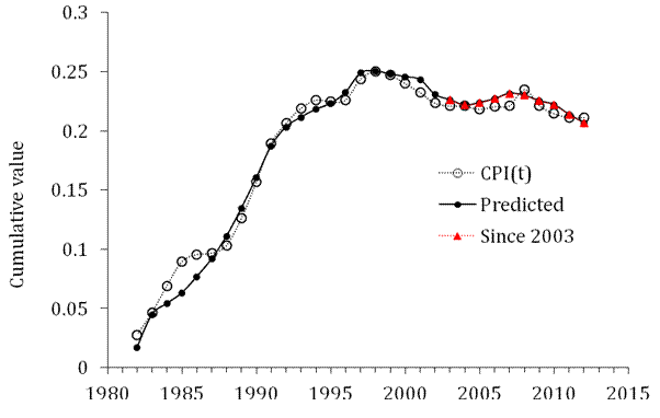
We have already mentioned that Japan is the best illustration of our concept linking inflation/unemployment to the change in labour force. In our previous post on the GDP deflator in Japan published a few days ago, we showed two cumulative curves for observed and predicted inflation since 1980. Here we revisit similar CPI curves also two more readings and conclude that our concept is quantitatively excellent. The underlying data have been borrowed from the OECD and Japan Statistics.  

Using stata9 and allowing a structural break, we sought for the best-fit (in RMS sense) coefficients in the linear and lagged link between inflation and labour force. Because of the structural (measurement related) break in the 1980s, we have chosen the period after 1981 for linear regression, which is common for almost all economic studies related to Japan. By varying the lag and coefficients we have found the following relationship for consumer price inflation (CPI): 

CPI(t) = 1.39dLF(t-t₀)/LF(t-t₀) + 0.0004           (1) 

where the time lag t₀=0 years; Figure 1 depicts this best-fit case. There is no time lag between the inflation series and the labour force change series in Japan. Free term in (1), defining the level of price inflation in the absence of labour force change, is close to zero but negative.  

A more precise and reliable representation of the observed and predicted inflation consists in the comparison of cumulative curves (a version of CUSUM technique) shown in the lower panel of Figure 1. We always stress that the cumulative values of price inflation and the change in labour force are the levels of price and labour force, respectively. Therefore, the summation of the annual reading gives the original estimates of price and workforce, which when are converted into rates.

 

Another advantage of the cumulative curves is that all short-term oscillations and uncorrelated noise in data as induced by inaccurate measurements and the inevitable bias in all definitions are effectively smoothed out. Any actual deviation between these two cumulative curves persists in time if measured values are not matched by the defining relationship. The predicted cumulative values are very sensitive to free term in (1).  

For Japan, the CPI cumulative curves are characterized by very complex and unusual for economics shapes. There was a period of intensive inflation growth and a long deflationary period. The labour force change, defining the predicted inflation curve, follows all the turns in the measured cumulative inflation with the coefficient of determination R²=0.99. The predicted and observed cumulative CPI curves are cointegrated and thus this estimate is consistent. For the annual estimates: R²=0.73.

 

With shrinking population, and thus, labor force, the level of CPI will be falling through 2050 and likely beyond.  

 

Figure 1. Measured CPI inflation and that predicted from the change rate of labour force in Japan. Upper panel:  Annual curves smoothed with MA(3). Lower panel: Cumulative curves between 1981 and 2012. The extremely accurate agreement between the cumulative curves illustrates the predictive power of our model. The cumulative curves are I(1) processes and  it was instructive to test them for cointegration. This test was successful.

What is the most efficient household size?

In my previous post, the evolution of mean family size was presented. In the same post, I also presented the long-term decrease in the mean household size from 2.89 in 1975 to 2.65 in 2011. The households break into smaller pieces as well as families. Here, we address the question of the most efficient size for a household. I propose to measure the efficiency in terms of income per person for a given household size. This measure might be not conventional but definitely explains the fall in the household size as the consequence of maximum income.

Figure 1 depicts seven curves of income per person (the average income for a given household size divided by the household size) for households of different sizes (10 people for the category 7+) normalized to the average household income (for all households) in a given year. The two people household is as efficient as one person household since 1998.  (Figure 2 depicts the same pattern for American families.)  Not surprisingly, the portion of one person and two people households increases rapidly since the start of measurement in 1975. These are two most efficient (in terms of personal income) household sizes. The portion of smallest households will rise in the future along their long term trends. Income rules!

Figure 1. Income per person for households of different sizes (10 people for the category 7+) normalized to the average household income in a given year.  

Figure 2. Income per person for families of different sizes (10 people for the category 7+) normalized to the average family income in a given year.

 

Figure 3. The portion of households of a given size since 1975.

Paid jobs break American families

In my previous post, the evolution of mean family size was presented. This size has been decreasing from 3.7 in 1965 to 3.13 in 2011 with the biggest families of 6 and more people splitting into smaller and smaller pieces. (All data were borrowed from the U.S. Census Bureau which is rich of data.).  I also showed that the portion of two people families observed from 1950 has a sustainable linear trend which will bring this portion to 50% by 2025. It’s sad news and the driving force behind these processes deserves a special consideration.

So, who is the family killer? I have a bit paradoxical answer. The American families started to break into smaller pieces when more people started to enter labor force.  Hence, a paid job is the reason for the families to split.  Figure 1 depicts the portion of five, six, and seven and more people families since 1950. It also shows the evolution of the participation rate in labor force, LFPR, reduced by 0.5 for the sake of comparison. In 1965, the LFPR started to grow together with the fall in the bigger families’ portion.  In 1990, both processes stopped and all curves reached some plateau.

The reason behind the current fall in the LFPR is of different nature and does not influence the family size much. There is no way back to bigger families.   

Figure 1. The portion of five, six, and seven and more people families compared to the participation rate in labor force. The start and amplitude of all processes are in an agreement.

American future – two people families

The U.S. Census Bureau is full of data. I was digging into the problem of the long term evolution of the household and family mean and median income and found a precious piece of measurements. Since 1950, the CB has been publishing the average size of family. For households, this data series is limited by 1975. Figure 1 shows the evolution of both variables. The family mean size was falling between ~1965 and 1990. (I would guess that the household size experienced a similar drop since 1965.) Since ~1990, there was no change beyond the measurement accuracy: 3.16 in 1988 to 3.16 in 2009 and 3.13 in 2011.

What is the reason behind the falling mean size?  Figure 2 depicts the evolution of the number of families of a given size (from 3 to 7+ ) normalized to the total number of families (from 2 people to 7+) in the USA. Figure 2 demonstrates that bigger families started to break into smaller pieces around 1965. The five people families still on a long term decline, but the share of 6 and 7+ people families stabilized around 1990. An immediate result of the split was the increasing share of 2, 3, and 4 people families between 1963 and 1990. However, the 3 and 4 people families started to break more intensively in 1990 and their shares have been on a negative  trend ever since.

Figure 3 shows the only winner of the breakage process – the two people families. By 2025, a half of American families will consist of 2 people!

Figure 1. The mean size of family and households in the U.S. as reported by the Census Bureau.

 

Figure 2. The shares of families with different sizes.

Figure 3. The share of 2 people families.

The most important message for Japan is that the overall level of prices associated with GDP is back to 1980 and the long term fall will continue into the next few decades.

We have already mentioned that Japan is the best illustration of our concept linking inflation/unemployment to the change in labour force. In our previous post on the GDP deflator in Japan in 2011, we showed two cumulative curves for observed and predicted inflation since 1980. Here we add two more readings in both curves and conclude that our concept is quantitatively excellent. It gives an extremely accurate long term equilibrium relation between the GDP deflator, DGDP, and labour force. The underlying data have been borrowed from the OECD and Japan Statistics.

 

The most important message for Japan is that the overall level of prices associated with GDP is back to 1980 and the long term fall will continue into the next few decades.

 

By trial-and-error, we seek for the best-fit coefficients in the linear and lagged link between inflation and labour force. Because of the structural (measurement related) break in the 1980s, we have chosen the period after 1981 for linear regression, which is common for almost all economic studies related to Japan. By varying the lag and coefficients we have found the following relationship: 

p(t) = 1.9dLF(t-t₀)/LF(t-t₀) – 0.0084         (1) 

where the time lag t₀=0 years; Figure 1 depicts this best-fit case. There is no time lag between the inflation series and the labour force change series in Japan. Free term in (1), defining the level of price inflation in the absence of labour force change, is close to zero but negative.  

A more precise and reliable representation of the observed and predicted inflation consists in the comparison of cumulative curves shown in the lower panel of Figure 1. We always stress that the cumulative values of price inflation and the change in labour force are the levels of price and labour force, respectively. Therefore, the summation of the annual reading gives the original estimates of price and workforce, which when are converted into rates.

Another advantage of the cumulative curves is that all short-term oscillations and uncorrelated noise in data as induced by inaccurate measurements and the inevitable bias in all definitions are effectively smoothed out. Any actual deviation between these two cumulative curves persists in time if measured values are not matched by the defining relationship. The predicted cumulative values are very sensitive to free term in (1). 

For Japan, the DGDP cumulative curves are characterized by very complex and unusual for economics shapes. There was a period of intensive inflation growth and a long deflationary period. The labour force change, defining the predicted inflation curve, follows all the turns in the measured cumulative inflation with the coefficient of determination R²=0.97 (R²=0.77 for the annual estimates). (Again, these are actually measured curves.) With shrinking population, and thus, labour force, the GDP deflator will be falling through 2050 and likely beyond.  

Figure 1. Measured GDP deflator and that predicted from the change rate of labour force in Japan. Upper panel:  Annual curves smoothed with MA(3). Lower panel: Cumulative curves between 1981 and 2012. The extremely accurate agreement between the cumulative curves illustrates the predictive power of our model.