Procter and Gamble - stable share price in Q4 2011

In this post, we revisit a share price model for Procter and Gamble as based on the decomposition into a weighted sum of two consumer price indices (to be determined), linear time trend and constant. It is shown that the model is valid since September 2009 at least and does not show any sign of possible failure. It predicts the share price at a four month horizon.

A share price model for Procter and Gamble (NYSE: PG) was originally published in this blog in July 2010. According to our concept, it was defined by the index of food away from home (SEFV - CUUS0000SEFV) and that of rent of primary residency (RPR); the evolution of these indices is presented in Figure 1. The former CPI component led the share price by 3 months and the latter one led by 8 months. The upper panel of Figure 2 depicts the original model and the monthly closing prices available in July 2010. This model was stable for the previous 11 months, i.e. for the period from September 2009.

In April 2010, we updated the original model using some new data (closing price for March 2011) and found that the same model was also applicable with a small change in the time lead for the SEFV – it was 4 months instead of 3 months in the original model. New coefficients were also slightly different, but very close to the original ones.

The most recent update uses the monthly closing price for September 2011 and CPIs for August 2011. It validates the model obtained for the previous period but is characterized by the same time lags and a small shift in the coefficients estimated by the LSQ technique. Three best-fit models for PG(t) are as follows:

PG(t) = -5.88SEFV(t-3) + 3.43RPR(t-8) + 17.60(t-1990) + 174.08, July 2010

PG(t) = -5.40SEFV(t-4) + 2.93RPR(t-8) + 18.16(t-1990) + 187.47, March 2011

PG(t) = -4.94SEFV(t-4) + 2.47RPR(t-8) + 18.15(t-1990) + 184.89, September 2011

where PG(t) is the monthly closing price (dividend and split adjusted) in US dollars, t is calendar time.

In the lower panel of Figure 2, the predicted curve leads the observed price by 4 months with the residual error of $2.12 for the period between July 2003 and September 2011 (see Figure 3 for the model residuals). In other words, the price of a PG share is completely defined by the behaviour of these two CPI components.

The model does predict the share price in the past and foresees a period of no growth in the fourth quarter of 2011. In January 2012, the price may fall, but we should revise the model with new data by that time.

Figure 1. Evolution of the price of SEFV and RPR.

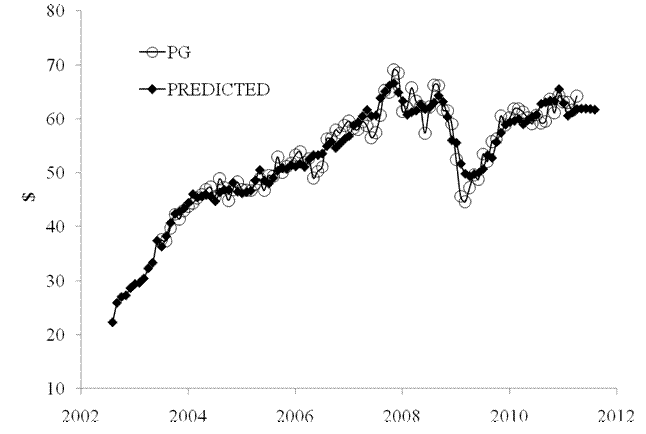
Figure 2. Observed and predicted PG share prices. In the upper panel, the original prediction published in July 2010 with a three month lead shown by red line. The middle panel – the model published in April 2011. The lower panel – the most recent model with the monthly closing price for September 2011.

Figure 3. The model residual error.

Loews Corporation share price in 2011 Q4

Half a year ago, we presented a share price model for Loews Corporation (NYSE: L) based on the decomposition into a weighted sum of two consumer price indices (selected from a larger number of CPIs), linear trend and constant, all coefficients and time lags to be estimated by a LSQ procedure. Here we test the previous model and make a regular update using new data. All in all, the original model is valid since October 2008 and does not show any sign of future changes. This is a reliable model valid during the past 47 months! 

A preliminary model for Loews Corp. was obtained in September 2009 and covered the period from October 2008. This old model included the index of food without beverages (FB) and the index of transportation service (TS). The most recent model also used the monthly closing prices as of April 2011 and the CPI estimates published on April 14, 2011. The defining indices were almost the same: the index of food (F) and the TS index. Figure 1 depicts the evolution of the indices which provide the best fit model, i.e. the lowermost RMS residual error, between October 2009 and September 2011.  The F index leads by 5 months and the TS index by 4 months.  When new data through September 2011 are used, the model does not show any tangible change - only coefficients have been slightly drifting: 

L(t) = -2.03F(t-5) – 2.12TS(t-4) +28.23(t-1990) + 448.98, March 2011

L(t) = -2.01F(t-5) – 2.09TS(t-4) +27.96(t-1990) +440.65, September 2011      

where L(t) is the share price in US dollars, t is calendar time. The new model is depicted in Figure 2 together with high and low monthly prices as a proxy to the uncertainty bound of the share price. The predicted curve leads the observed one by 4 months. The residual error is of $2.38 for the period between July 2003 and September 2011.  In the fourth quarter of 2011, the model foresees a very slight increase. The model obtained in March 2011, accurately predicted the fall observed in the second and third quarters.   

Figure 1. Evolution of the price indices F and TS.

Figure 2. Observed and predicted share prices.

On the evolution of Forest Laboratories stock prices

During the past two days, we re-estimated share price models for a few companies from the S&P 500 list and found them reliable and accurate for a year and even longer. Forest Laboratories (NYSE: FRX) is one of the first companies with a stable and deterministic share price modelestimated in September 2009 (this early model tracks back into November 2008).  This is a company from Healthcare subcategory specialized in drugs manufacturing. We revisited this model in September 2010, December 2010, and March 2011 and always found the same defining variables with almost the same time lags.  

Our approach to deterministic share pricing is based on the decomposition of a share price into a weighted sum of two selected consumer price indices. For FRX, all models between 2009 and 2011 are defined by the (not seasonally adjusted) index of dairy and related products (DAIRY) and the price index of other household equipment and furnishing (OHEF), as reported by the US BLS. In the September 2011 model, the former CPI component leads the share price by 4 month and the latter is 5 months ahead of the share price. Figure 1 depicts the overall evolution of both involved indices through August 2011.  

Thus, three models mentioned above are as follows: 

FRX(t) =  -0.53DAIRY(t-3) – 4.18OHEF(t-5)  - 13.41(t-1990) + 706.57 (September 2009)   

FRX(t) =  -0.61DAIRY(t-3) – 3.89OHEF(t-4)  - 11.65(t-1990) + 668.75 (March 2011) 

FRX(t) =  -0.66DAIRY(t-4) – 3.45OHEF(t-5)  - 9.78(t-1990) + 613.99 (September 2011)     

where t is calendar time. All coefficients have been slightly drifting due to then trade-off between the linear time trend and the trend in the difference between the CPIs and due to new data. Therefore, the model is effectively the same between November 2008 and September 2011. In other words, we obtained a deterministic (leading by three months) model which was valid during 36(!) months.   Figure 2 depicts the predicted and observed prices together with the relevant monthly highs and lows. The residual error is $4.75 (see Figure 3) for the period between June 2003 and September 2011 ($4.40min March 2011). From the most recent model in Figure 2, we expect a fall to the level of $20 per share in the fourth quarter of 2011.  

Figure 1. Evolution of the price of DAIRY and OHEF. 

Figure 2. Observed and predicted FRX share prices. 

Figure 3. The model residual.  

BofA, how are you doing?

Twenty months ago we presented a preliminary share price model for Bank of America (NYSE: BAC). It was based on the decomposition of the price into a weighted sum of two consumer price components, a linear time trend and a constant (see details here). All coefficients, time lags and CPIs were estimated by the least squares as applied to the model error.   Here we revisit the model using new data through September 2011. The newly estimated model differs from the preliminary one due to strict constraints on time lags and new data.

The preliminary model was a defined by the index of food without beverages (FB) and that of food away from home (SEFV). The latter CPI component leads by 13 months. From our past experience, the larger is the lag the more unreliable is the model. So it happened to the preliminary model and the best-fit two component model for BAC(t) is as follows:  

BAC(t)= -2.35OHF(t) + 1.19H(t) + 1.97(t-1990) + 165.79

   

where OHF is the consumer price index of other food at home and H(t) is the index of housing, both having notime lag behind the price (see Figure 1 for the evolution of the CPIs). Both CPIs are available only for August 2011, and thus we actually have a one month lead of the CPIs, if they would have been already available for September 2011. One has to reestimate the model when the CPIs for September are published by the BLS . The standard deviation of the modeling error is $2.80 for the period between July 2003 and September 2011.

Figure 2 depicts the observed and predicted prices and indicates that the market overestimates the share above the predicted level. The overestimation is also clear from Figure 3 where the model residual is displayed. All in all, Bank of America might have serious problems, which could bring its share price down to $1 in the near future. Similar problems had Lehman Brothers and other banks several months before bankruptcy. BofA aslo was a bankrupt, but    was bailed out.

Figure 1. The evolution of the defining consumer price indices.

Figure 2. Observed and predicted BAC share prices. 

Figure 3. The model error

Aflac may grow to $45 in December 2011

Here we revisit the stock price model for Aflac Incorporated (AFL) which we obtained in April2011 using our concept of share pricing. Accordingly, our goal is to test the original model and to update time lags and coefficients.

Last time we predicted the AFL price using the CPI estimates published by the BLS for March 2011. It was a preliminary model.  The share price was defined by the consumer price index of household furnishing and operations (HFO) and that transportation services (TS). The defining time lags are as follows: the HFO index led the share price by 2 months and the TS by 4 months. Adding new data for the period between April and September 2011, we re-estimated the model and found some changes in the time lags: zero and five months, respectively; and in the estimated coefficients. The relevant best-fit 2-C models for AFL(t) are as follows: 

AFL(t) =  -5.02HFO(t-2) – 2.87TS(t-6)  + 20.42(t-1990) + 997.71,  March 2011

AFL(t) =  -4.63HFO(t-0) – 2.90TS(t-5)  + 20.41(t-1990) + 953.49, September 2011 

where AFL(t) is the AFL share price in U.S. dollars,  t is calendar time. The changes in time lags are shown in red.  

In July2011, we reported that the original model gave a correct prediction of the fall in Q2 2011. Here we show that the current fall in the price has to stop and expect a positive correction in Q4 2011. Figure 1 depicts the high and low monthly prices for an AFL share together with the predicted and measured monthly closing prices (adjusted for dividends and splits). As a rule, the predicted prices are well within the bounds of the share price uncertainty.  However, the price has fallen too much in Q3 and the model residual error (Figure 2) is negative what indicates a positive correction any time soon, if the model is right.  

Figure 1. Observed and predicted AFL share prices. 

Figure 2. The model residual error.

Alcoa share price may fall to $5 in December

Six months ago we reported a share price model for Alcoa (AA), which is company from Materials subcategory of the S&P 500 list specialized in aluminum. Here we test and update the model using new data, including the monthly closing price in September 2011 and the estimated CPI components for August. The principal result is that we accurately predicted the behavior in Q2 and Q3 and the updated model has the same defining CPI components and time lags with slightly shifted coefficients. Therefore, the model is a reliable tool to predict the evolution of Alcoa at a two month horizon.

According to our general approach to share price modeling we decompose the observed time history of the monthly closing AA stock price (adjusted for splits and dividends) into a weighted sum of two CPI components, time trend and free term.  Two defining CPI components are selected to minimize the model (RMS) error and may lead or lag behind the share.  

The original and current AA model is defined by the (not seasonally adjusted) index of food away from home (SEFV) and the price index of rent of primary residence (RPR), as reported by the US BLS. The former CPI component leads the share price by 2 months and the latter is 4 months ahead of the share price. Figure 1 depicts the overall evolution of both involved indices through August 2011. It seems these indices have been evolving in sync since 2002 with the only step-like change in the SEFV index in 2008.  We present two empirical models as estimated in April and October 2011: 

AA(t) =  -6.71SEFV(t-2) + 3.34RPR(t-4)  + 19.23(t-1990) + 298.87, Aril 2011

AA(t) =  -6.61SEFV(t-2) + 3.22RPR(t-4)  + 19.51(t-1990) + 300,89, October 2011 

where AA(t)  is a share price in US dollars, t is calendar time. Figure 2 illustrates the observed and predicted models for October 2011. The residual error is $3.04 ($3.12 in April) for the period between July 2003 and September 2011. Figure 2 also shows monthly high and low prices as the uncertainty in the monthly closing price as the best share price estimate. Since the closing price has to characterise the whole month by one value the high and low prices might serve as statistical bounds.  

One can expect the share price to fall to the level of $5 in December 2011. 

 

Figure 1. Evolution of the price of SEVF and RPR. 

Figure 2. Observed and predicted AA share prices.  

Predicting Harley-Davidson share price

Harley-Davidson (HOG) is one of the best illustrations of our concept (see a brief description of the concept in Appendix) linking stock prices to CPI components. For HOG, the model is stable for many years. The first model was obtained in September 2009 and covered the period from October 2008. Here we revisit the HOG model using the monthly closing price for September 2001 and the CPI estimates published for August 2011.  

For HOG, the defining indices are as follows: the index of rent of primary residence (RPR) and the index of owners' equivalent rent of residence (ORPR). Both CPI components are leading the share price. Figure 1 depicts the evolution of the indices which provide the best fit model, i.e. the lowermost RMS residual error, between July 2008 and September 2011.  The models are as follows: 

HOG(t) = -13.82RPR(t-3) +12.77ORPR(t-4) +17.82(t-1990) – 163.94, before September 2009

HOG(t) = -11.30RPR(t-3) + 9.83ORPR(t-3) +17.53(t-1990) – 36.34, July 2011

HOG(t) = -11.27RPR(t-3) + 9.55ORPR(t-3) +19.35(t-1990) – 8.57, September 2011 

where HOG(t) is the share price in US dollars, t is calendar time. The model is characterised by standard deviation of $4.33 for the period between July 2003 and September 2011.   

Two recent models are depicted in Figure 2. The predicted curves lead the observed ones by 3 months. We do not foresee any further fall in the stock price.  Figure 3 displays the residual error.

Figure 1. Evolution of the price indices ORPR and RPR.

Figure 2. Observed and predicted POM share prices. Upper panel – the model for March 2011. Lower panel – the model for September 2011.

Figure 3. The model residual error.  

Appendix

In its general form, our pricing model is as follows: 

sp(t_j) = Σb_i∙CPI_i(t_j-t_i) + c∙(t_j-1990 ) + d + e_j                                                              (1) 

where sp(t_j) is the share price at discrete (calendar) times t_j, j=1,…,J; CPI_i(t_j-t_i) is the i-th component of the CPI with the time lag t_i, i=1,..,I; b_i, c and d  are empirical coefficients of the linear and constant term; e_j is the residual error, which statistical properties have to be scrutinized. By definition, the bets-fit model minimizes the RMS residual error. The time lags are expected because of the delay between the change in one price (stock or goods and services) and the reaction of related prices. It is a fundamental feature of the model that the lags in (1) may be both negative and positive. In this study, we limit the largest lag to eleven months. Apparently, this is an artificial limitation and might be changed in a more elaborated model.

System (1) contains J equations for I+2 coefficients. For POM we use a time series from July 2003 to March 2011, i.e. 94 monthly readings.  Due to the negative effects of a larger set of defining CPI components their number for all models is (I=) 2. To resolve the system, we use standard methods of matrix inversion. As a rule, solutions of (1) are stable with all coefficients far from zero. In the POM model, we use 92 CPI components. They are not seasonally adjusted indices and were retrieved from the database provided by the Bureau of Labor Statistics.

Due to obvious reasons, longer time series guarantee a better resolution between defining CPIs. In general, there are two sources of uncertainty associated with the difference between observed and predicted prices. First, we have taken the monthly close prices (adjusted for splits and dividends) from a large number of recorded prices: monthly and daily open, close, high, and low prices, their combinations as well as averaged prices. Second source of uncertainty is related to all kinds of measurement errors and intrinsic stochastic properties of the CPI and its components. One should also bear in mind all uncertainties associated with the CPI definition based on a fixed basket of goods and services, which prices are tracked in few selected places.  Such measurement errors are directly mapped into the model residual errors. Both uncertainties, as related to stocks and CPI, also fluctuate from month to month.