Okun’s law revisited. Is there structural unemployment in developed countries?

Abstract

Okun’s law for the biggest developed countries is re-estimated using the most recent data on real GDP per capita and the rate of unemployment. Our results show that the change in unemployment rate can be predicted with a high accuracy. The link needs the introduction of a structural break which might be caused by the change in monetary policy or/and in measurement units. Statistically, the link between the studied variables is characterized by the coefficient of determination between 0.40 (Australia) and 0.84 (the USA). The residual errors can be associated with measurement errors. The obtained results suggest the absence of structural unemployment in the studied developed countries.

Key words: unemployment, GDP, modelling, Okun’s law

JEL classification: J65 

Introduction

The Sveriges Riksbank Prize in Economic Sciences in Memory of Alfred Nobel 2010 was awarded to P. Diamond, D. Mortensen and C. Pissarides ”for their analysis of markets with search frictions”. The core result of their study was an explanation of labour market dynamics including unemployment (e.g. Diamond, 2011; Mortensen and Nagypal, 2007; Pissarides, 2000). Hence, the dynamics of unemployment is a very important and actual problem for the modern economics.

One of the most actively discussed topics related to unemployment is its high persistence since the start of the financial crisis. In the United States, the current rate unemployment is above 9% and it does not show any sign of reduction in the future. There is an opinion that the current situation might manifest tangible structural changes in the labour market. This implies some major changes in the overall organization of the economy when significant parts of it become unnecessary.

We address the problem of structural unemployment by modelling the rate of unemployment using the relationship explaining the dynamics of unemployment by its negative correlation with the growth in GDP – Okun’s law (1962). This relation was revisited many times in the past (e.g. Altig, Fitzgerald and P. Rupert, 1997; Knotek, 2007; Tillman, 2010).

We also revisit Okun’s law using the most recent data on GDP per capita provided by the Conference Board (2011) and data on unemployment from the OECD (2011). To improve the agreement between the change in unemployment rate and real GDP per capita we introduce structural breaks in Okun’s law. Such breaks might manifest artificial changes in definitions of unemployment and real GDP as well as actual shifts in the linear relationship.

We have assessed Okun’s law in the biggest developed countries: the United States, France, the United Kingdom, Australia, Canada and Spain. Our results suggest the absence of structural unemployment in the studied developed countries. The persistence of high unemployment is completely related to low rate of real economic growth. In all studied countries, the rate of growth above 2% per year will result in a fall of the unemployment rate.

Okun’s law and empirical results

According to the original form of Okun’s law, there exists a negative relation between the growth rate of real GDP and the change in unemployment rate, du=u_i-u_i-1. The overall GDP includes the change in population as an extensive component which is not necessary dependent on other macroeconomic variables. Econometrically, it is mandatory to use macroeconomic variables of the same origin and we use real GDP per capita, G. It is better related to the portion of labor force without job, i.e. the rate of unemployment. Therefore, we rewrite Okun’s law in the following form:

            du = a + bdlnG      (1)

where dlnG=dG/G is the relative change rate of real GDP per capita, a and b are empirical coefficients.  Okun’s law suggests that b<0.  

We start with the United States and have to introduce a structural break in 1984 into the link. The following relationship was obtained:  

 du = -0.42dlnG + 1.07, t<1985

 du = -0.62dlnG + 1.09, t>1984             (2) 

where dlnG in the annual growth rate of real GDP per capita, du is the annual increment in the rate of unemployment, u. Figure 1 displays the observed and predicted du between 1958 and 2010. The agreement is excellent. Figure 2 presents some regression results for the curves in Figure 1 with the coefficient of determination R²=0.84. Therefore, more than 84% of the variability in the change of unemployment rate in the U.S. is explained by the change in real GDP per capita. Considering the fact that both macroeconomic variables are measured with an accuracy of approximately 1 percentage point the residual 16% of the variability can be easily associated with the uncertainty in their measurements. Figure 3 demonstrates that the residual error is rather random and does not contain a unit root and has no significant autocorrelation.

Relationship (2) shows that the sensitivity of the du to dlnG becomes higher after 1984 with the slope of -0.62 and the intercept +1.09. There are two assumptions on the reasons behind this structural break. One is related to the changes in monetary policy in the early 1980s to overcome extremely high inflation. On the other hand, the measures of the GDP deflator and CPI start to deviate around 1980 and the rate of unemployment obtained a new definition in 1984. Thus, the shift in 1984 might also be associated with new units of measurements. In any case, the period after 1984 is described with a very high accuracy including three episodes of unemployment surge in 1991, 2001 and 2009. Moreover, relationship (2) provides a smooth transition through 1984 and describes the fall in unemployment in 1984.

We have also checked several macroeconomic variables as a predictor variable in Okun’s law: the overall GDP, GDP per capita corrected for the difference between the whole population and working age population, and productivity as expressed by real GDP per worker.  All these variables are inferior to real GDP per capita and thus we use this variable for other countries.

The next country to model is France. We have reversed (1) and obtained the following relationship for dlnG:  

 dlnG = -5.0du + 4.6, t<1987

 dlnG = -1.5du + 1.4, t>1986                      (3)

Figure 4 present the observed and predicted curves. There is a shift in the dependence around 1987 and the slope in (3) fell from -5.0 to -1.5.  Correspondingly, the sensitivity of the unemployment rate to real GDP growth (the reciprocal value of the slope in (3)) increased from -0.2 to -0.67. In order to decrease the rate of unemployment in France, real GDP per capita has to grow by 1.5% per year. When the growth rate is lower, the rate of unemployment increases. 

For France, both variables are characterized by an elevated volatility and thus the coefficient of determination R²=0.53 is relatively low. To remove the measurement noise we have smoothed both curves with MA(3). The lower panel in Figure 4 shows that the agreement between the measured increase in real GDP per capita and that predicted from the change in unemployment rate became extremely good.  

The United Kingdom also shows an excellent result for Okun’s law. The following equation:

dlnG = -1.5du + 2.5, t<1987

dlnG = -2.0du + 1.7, t>1986                 (4) 

describes the period after 1972. Figure 5 illustrates the agreement between the observed and predicted time series. Before 1972, the OECD provides no unemployment estimates. The year of structural break is the same as in France but the change in the slope is much lower. In any case, to reduce the current rate of unemployment the UK needs to grow at a rate above 1.7% per year in term of real GDP per capita.  

For Canada, the following equation was estimated with a structural break around 1985:  

dlnG = -2.7du + 3.1, t<1985

dlnG = -2.7du + 1.2, t>1984       (5) 

Figure 6 depicts the measured and predicted curves for dlnG. For Canada, the rate of growth above 1.2% per year is enough to reduce the rate of unemployment from its current level of 8%. In 2009, dlnG=-0.033 y^-1 and the rate of unemployment rose by 4.7%. In 2010, the change rate of real GDP per capita was +0.021y^-1 and the rate of unemployment fell by 0.3%.   For Australia, the following equation was estimated with a structural break around 1995:  

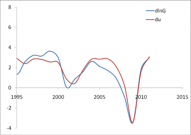
dlnG = -1.7du + 2.4, t<1995

dlnG = -3.0du + 1.2, t>1994       (6) 

The timing of this break is different from those obtained before but the shift in the slope and intercept is big enough to consider it with confidence. It is likely that the structural break was induced by the introduction of a new monetary policy in 1994 (RBA, 1994).

 

Figure 1.  The link between the du and dlnG in the U.S. as described by relationship (2) with a structural break in 1984 

Figure 7 displays the measured and predicted curves for dlnG. The overall agreement is not good with R²=0.40 for the period between 1968 and 2010. This low correlation coefficient is associated with the high volatility in both time series. When smoothed with MA(3), the curves in Figure 7 show a much better resemblance. For Australia, the rate of growth above 1.2% per year is enough to reduce the rate of unemployment from its current level of 5.2% (2010). It is similar to Canada. 

Finally, the case of Spain is a decisive one. The rate of unemployment in Spain is extremely high and has been varying in a wider range since the 1960s. This is a big challenge for Okun’s law. We have obtained the following relationship with a structural break in 1987:  

dlnG = -2.0du + 5.0, t<1987

dlnG = -0.8du + 2.1, t>1986                     (7) 

The timing of this break practically coincides with those in other countries. The sensitivity of unemployment to real economic growth rose significantly in 1987. 

Figure 8 displays the measured and predicted curves for dlnG. The overall agreement is not good with R²=0.59 for the period between 1961 and 2010. When smoothed with MA(3), the curves in Figure 8 show an extraordinary agreement but one can also introduce another structural break near 1968.

Figure 2.  A scatter plot du against dlnG from Figure 1with a linear regression line. R²=0.84.

Figure 3. The model error for the U.S.

Figure 4.  Observed and predicted dlnG for France. The lower panel presents the curves smoothed with MA(3).

Figure 5.  Observed and predicted dlnG for the UK. The lower panel presents the curves smoothed with MA(3). 

Figure 6.  Observed and predicted dlnG in Canada. The lower panel presents the curves smoothed with MA(3).

Figure 7.  Observed and predicted dlnG in Australia. The lower panel presents the curves smoothed with MA(3).

Figure 8.  Observed and predicted dlnG in Spain. The lower panel presents the curves smoothed with MA(3).

Conclusion

With real GDP per capita instead of the overall GDP, Okun’s law demonstrates an extraordinary predictive power for the biggest developed countries. One can accurately describe the dynamics of unemployment since the 1960s. The currently high levels of unemployment in developed countries cannot be reduced without fast economic growth well above 2% per year. In that sense, there are no structural unemployment components in the currently high rates of unemployment in the studied countries. 

References

Altig, D., T. Fitzgerald, and P. Rupert. (1997). Okun’s Law Revisited: Should We Worry About Low Unemployment?” Federal Reserve Bank of Cleveland, Economic Commentary.

Conference Board. (2011).  Total economy database. http://www.conference-board.org/data/economydatabase/

Diamond, P. (2011). Unemployment, Vacancies, Wages. American Economic Review, 101(4): 1045–72.

Knotek, E. S. II. (2007). How Useful is Okun’s Law?, Federal Reserve Bank of Kansas City Economic Review, 4th Quarter, 73-103.

Mortensen, D. T. and E. Nagypal. (2007). More on Unemployment and Vacancy Fluctuations, Review of Economic Dynamics, 10 (3): 327{347.

Okun, A. M. (1962). Potential GNP: Its Measurement and Significance, American Statistical Association, Proceedings of the Business and Economics Statistics Section, 98–104.

Organization of Economic Cooperation and Development (2011). Original release data and revisions database. http://stats.oecd.org/mei/default.asp?rev=1

Pissarides, C. A. (2000). Equilibrium Unemployment Theory, Cambridge: MIT.

Reserve Bank of Australia. (1994). 1994 Report and Financial Statements. Reserve Bank of Australia. Sydney

Tillmann,  P. (2010). Do FOMC members believe in Okun's Law? Economics Bulletin,  30, No. 3, 2398-2404.

Modeling the change in unemployment rate: Canada, Australia and Spain

I continue model the change in unemployment rate as a linear function of the change rate  of real GDP per capita. (See my previous posts)

For Canada, I have estimated the following relation with a structural break in 1985

dlnG = -2.7du + 3.1, t<1995

dlnG = -2.7du + 1.2, t>1994

Figure 1 presents the observed dlnG curve and the scaled du, i.e. the change in GDP predicted from the change in the rate of unemployment.  The agreement is excellent, but both curves are volatile. I have smoothed them with MA(3).

For Spain, the result is really fantastic! the following relation is obtained with a structural break in 1987:

dlnG = -2.0du + 5, t<1987

dlnG = -0.8du + 2.1, t>1986

Figure 2 presents the observed and predicted dlnG. There might be another structural breal around 1970.

For Australia, the result might be not so exciting but is very good:

dlnG = -1.7du + 2.5, t<1995

dlnG = -3.0du + 1.3 t>1994

Figure 3 presents the observed and predicted curves smoothed with MA(3) and a structural breal in 1995. 

Figure 1. Annual growth rate of real GDP per capita, dlnG, and the scaled rate of unemployment, du. The lower panel shows the curves smoothed with MA(3)

Figure 2. Same as in Figure 1 for Spain .

Figure 3. Same as in Figure 1 for Australia

On the link between real growth and rate of unemployment again

My previous post was very exciting. Not every day one can find highly correlated economic time series.  The first move was to introduce a structural break into the link between the change in unemployment rate, du, and the change rate of GDP per capita, dlnG. In my previous post, I have found the following relationship:

                 dlnG = -2.4du+2.25

where dlnG  in the annual growth rate of real GDP per capita, du is the annual increment in the rate of unemployment, u. It also was shown that the sensitivity of the du to dlnG becomes lower after 2000, and the slope of -1.6 and the intercept of 2.1 better describe the link.   Actually, there is a structural break around 1984 and the new relationship is as follows

dlnG = -1.6du + 1.75, t>1984

Figure 1 depicts the predicted (with a structural break) dlnG and scaled du. Figure 2 presents regression results with Rsq.=0.84.  The agreement is more than exiting – it is breathtaking.

There is a more urgent question. Does it work for other developed countries? The answer is yes!

For France, I have estimated the following relation with a structural break in 1987

dlnG = -5.0du + 4.6, t<1987

dlnG = -1.5du + 1.4, t>1986

Figure 3 presents the observed dlnG curve and the scaled du, i.e. the change in GDP predicted from the change in the rate of unemployment.  The agreement is excellent, but both curves are volatile. I have smoothed them with MA(3).

For the UK, the following relation is obtained with a structural break in 1987:

dlnG = -1.5du + 2.5, t<1987

dlnG = -2.0du + 1.7, t>1986

Figure 4 presents the observed and predicted dlnG. The OECD reported the rate of unemployment only after 1972 for the UK.

Paul Krugman is right. One should not expect the rate of unemployment to fall before the rate of real GDP growth will exceed 2-3% per year in the US, UK and France.

Figure 1. Annual growth rate of real GDP per capita, dlnG, and the scaled rate of unemployment, du.

Figure 2. Scatter plot of the curves in Figure 2 and linear regression.

Figure 3. Same as in Figure 1 for France . The lower panel shows the curves smoothed with MA(3)

Figure 4. Same as in Figure 1 for the UK

Bravo, Krugman!

A month ago I presented a graph linking the growth rate of real GDP per capita and the rate of unemployment. Figure 1 is borrowed from this post and shows that one can expect the rate of unemployment to  fall fast in the second half of 2011.

Figure 1. The annual change rate of real GDP, dlnGDP/dt, and the scaled rate of unemployment, UE.

Paul Krugman has modified this graph in order to prove that the current  rate of unemployment is a direct consequence of slow real growth. He plotted the change in unemployment rate against the change rate of real GDP.  In his scatter plot, correlation was very high.  I decided to repeat his result using GDP per capita instead of the overall GDP, which is a biased measure of growth in econometric assessments.  The only thing I have to say:

Bravo, Krugman!

This is almost the best economic graph I have ever seen. Figure 2 presents it in my interpretation and shows that the change in unemployment rate, du, almost coincides with the change rate of GDP per capita, dlnG. In Figure 2, we have scaled the du with the following relationship:

dlnG = -2.37du+2.25

or

du= -0.42 dlnG + 0.95

Figure 3 presents results of regression: Rsq.=0.81. For the scaled du, the slope is 1.0.

However, the current fall in the rate of unemployment exceeds the predicted one. Somehow, the sensitivity of the du to dlnG becomes lower after 2000, and the slope of -1.6 and the intercept of 2.1 better describe the link.  For these values of slope and intercept, the rate of real economic growth, dlnG, should be ~2% per year for the rate unemployment retained at 9.6%. For the rate of unemployment to fall, one needs the real growth rate above 2% per year.

Figure 1 looks a bit biased. We have also to reconsider this post on unemployment as based on the change in labor force, which predicted the rate of unemployment around 8% in 2012.

Figure 2. Annual growth rate of real GDP per capita, dlnG, and the scaled rate of unemployment, du.

Figure 3. Scatter plot of the curves in Figure 2 and linear regression.

Figure 4. Same as in Figure 2 with the slope -1.5 and intercept +2.0 for the period after 1995.

Is the mainstream economics a science?

I like to collect citations from well-known economists. They actually think that economics is a hard science and they are scientists in terms of methodology.  Sometimes they give direct examples and compare economics with some hard sciences. This is one of examples from R.Schiller who compares economics and medicine:
Imagine how the medical profession would view one of its members who recommended to the general public some therapy that had not yet passed scrutiny from the appropriate authorities. Medical professionals know how often seemingly promising new therapies turn out, after careful study, not to work, or even to be harmful. There is a rigorous process of scholarly review of proposed new therapies, associated with professional journals that uphold high research standards. Circumventing that process and promoting new, untested ideas to the general public is unprofessional.
By irony, Robert explains the difference between the medical profession and economists in the very beginning of his post:
... An apparent paradox emerged from the discussion: the boom in popular economics comes at a time when the general public seems to have lost faith in professional economists, because almost all of us failed to predict, or even warn of, the current economic crisis, the biggest since the Great Depression.

Imagine now that the medical profession has the same "success" in the main fields of research. Would anybody go to a  doctor at all?  What were the criteria of " ... scrutiny from the appropriate authorities"  in the economics profession?

Please, do not steal from the hard sciences the merits economics does not deserve. There is no scientific methodology in the current economic knowledge because economits explicitly deny the necessity to compare observations and predictions. This is the core of medical scrutiny.  If to compare an economist and a doctor, the former should never approach the patient.

On the healthy growth in employment

After the employment  report for June, a number of bloggers (e.g. Mark Thoma and David Leonhardt ) suggested that a healthy monthly  increment in employment would be between 100,000 and 150,000. I have addressed this issue in my previous post as  well. The current employment/population ratio is aproximately 58%. One should notice that only people of 16 years of age and over are counted in.
On avearge, this civilian population has been growing since January 2010 by 143,00 per month. With the rate of 0.58 one would expect 83,000 per month. Actually, the increment since January 2010 is 76,000 per month . This estimate is from household employment data, i.e. the same source as for the civilian population.  The difference of 6,000 can not be considered as a dramatic one.

A responsible commenter should check actual data.

Is the employment situation really disappointing? II

This post almost completely repeats our post on employment situation a month ago.

The Bureau of Labor Statistics has published an “Employment Situation Summary” for June. The nonfarm payroll employment has increased by 18,000 (establishment data). The number of employed in the U.S. has decreased by 445,000; from 139,779,000 to 139,334,000 (household data).  As in May 2011, these low numbers have come as a surprise for many experts, who expected 105,000 for the nonfarm payroll employment in June.

We have already demonstrated that the level of labor force in the U.S. has been experiencing an unprecedented fall since 2008. Figure 1 reminds us that the reason for the fall is not the current financial crisis and recession but rather a new trend in the rate of labor force participation, LFP. This is not a short- or mid-term transient process but the change in the long-term tendency. The LFP had been growing between 1955 and 2000, when it reached its peak. One can consider 2001 as a pivot point manifesting a fundamental change in the labor market behavior in the U.S. It is worth noting that the change in LFP behaviour started ten years ago, not in 2008. (The reader might be interested in the explanation of this phenomenon. We had accurately predicted the 2010/2011 fall in the LFP many years before it happened.)

As a result of the new long-term tendency, one should not expect the same pace of employment growth as it was between 1960 and 2000. In addition to the fundamental shift in the secular LFP evolution, one should not forget another source of employment growth – the level of working age population. Figure 2 depicts monthly increments of the working age population, i.e. 16 years old and over.  One can clearly see that the influx of the population has been decelerating since 2000 as well. The deep negative corrections in Figure 2 are associated with annual revisions to population controls. It is not wise to wait that the growth in employment will exceed the influx of working age population in the situation with the falling LFP.    

It is important that even decreasing unemployment can not compensate the effects of LFP and population. Figure 3 shows the evolution of monthly increments in employment, E, after 2003 with MA(12). One should not expect that E will be growing at a pace which was considered as a healthy one before 2000 any time soon. As a month before we can conclude that the today’s BLS figures are not disappointing. Really disappointing is the unjustified expectation of any large increase in the U.S. employment.  

Figure 1. Measured LFP in the U.S.

Figure 2. Monthly increment in working age popualtion (16 years of age and over) in the U.S.

Figure 3. Monthly increment of employment in the US with its MA(12).