Economics as Classical Mechanics

4/23/11

Does crude drive the price index of steel and iron? (update)

We have been following the link between price indices of iron&steel and crude oil (domestic production) since 2009. This is a quarterly update. The previous update included PPI data as of November 2010. Here we extend the set by data available after April 13, 2011. Otherwise, we retain the form of the report untouched.

Historically, we first reported that the price index of crude oil had been likely evolving in sync with that of iron and steel, but with a lag of two months in September 2009 [1]. In order to present both indices in a comparable form, the difference between a given index, iPPI (i.e. iron&steel and crude), and the overall PPI was normalized to the PPI: (iPPI(t)-PPI(t))/PPI(t). The normalized differences represent the evolution of the rate of deviation from the PPI over years.

Figure 1 depicts the corresponding time histories of the normalized deviations from the PPI, including the most recent period since December 2010. Simple visual inspection reveals the following feature: the (normalized deviation from the PPI of the) index of iron and steel lags by approximately two months behind the (normalized) index of crude oil.

Figure 1. The deviation of the iron and steel price index and the index of crude oil from the PPI, normalized to the PPI.

In order to reduce both deviations to the same scale we additionally normalized the curves in Figure 1 to their peak values between 2005 and 2011

(iPPI(t)-PPI(t))/[PPI(t)*max{iPPI-PPI)}]

This scaling allows a direct comparison of corresponding shapes. In Figure 2, we display the normalized index of iron and steel shifted by two months ahead to synchronize its peak with that observed in the normalized index for crude petroleum. The scaled index of crude demonstrates just short-term deviations from the index of iron and steel in the overall shape and timing of the peak and trough. Simple smoothing with MA(3) makes the curves resemblance even better. As an invaluable benefit of the resemblance, one can use the two-month lag to predict the future of the iron and steel price index.

Figure 2. Deviation of the iron and steel price index from the PPI, normalized to the PPI and the peak value after 2005 as compared to the deviations of the index for crude petroleum normalized in the same way. The normalized index for iron and steel is shifted two months ahead.

Conclusion

Between 2006 and 2011, the deviation of the price index of iron and steel from the PPI in the USA repeats the trajectory of the deviation of the index of crude petroleum (domestic production) with a two-month lag. Therefore, the prediction of iron and steel price for at this horizon is a straightforward one.

References

1. Kitov, I., Kitov, O., (2009). Sustainable trends in producer price indices, Journal of Applied Research in Finance, Spiru Haret University, Faculty of Financial Management and Accounting Craiova, vol. I(1(1)_ Summ), pp. 43-51

Yahoo! share in Q2 2011

In January 2011, we wrote about YHOO share in 2011 Q1:

Currently, the predicted price shows no tendency to rise. All in all, one should not expect the YHOO price to grow fast.

This prediction was right and YHOO shares stalled in Q1. Here we update the underling model and give a forecast for 2011Q2.

Since the last revision in January 2011, the model for Yahoo! (YHOO) had no significant changes and still is a slightly weird example of the deterministic character of share price evolution. The YHOO model is stable over the past year and a half and is defined by somewhat unexpected indices: the consumer price index of meat, poultry, fish and eggs (MEAT) and the index of motor vehicle parts and equipment (MVP). Both defining indices seem to have no visible relation to the internet services. On the other hand these CPIs are the most basic ones and are in the root of any economic activity.

In the new model, the MEAT index leads the share price by 5 months (6 months in January) and the MVP has no lead (1 month in January). Figure 1 depicts the overall evolution of both involved indices. These two defining components provide the best fit model between June 2010 and March 2011. The MEAT coefficient is positive and thus the increasing price of meats, poultry, fish and eggs causes the share price to grow at a slow pace. The MVP index has a negative coefficient and causes the share to fall. The slope of time trend is positive revealing the price tendency to increase over time. The best-fit 2-C model for YHOO(t) is as follows:

YHOO(t) = 0.49MEAT(t-5) – 3.25MVP(t-0) + 10.66(t-1990) + 145.61

where YHOO(t) is the price of a share in US dollars, t is calendar time.

The predicted and observed curves are presented in Figure 2. The residual error is of $2.56 for the period between June 2003 and March 2011 (see Figure 3). In the second quarter of 2011, the price of food will likely be growing and the MVP has a tendency to fall. This may introduce a positive force into the share and it will be growing through the quarter.

Figure 1. Evolution of the price of MEAT and MVP.

Figure 2. Observed and predicted YHOO share prices.

Figure 3. The model residual. Currently, the price is underestimated.

4/22/11

COP, XOM, CVX, DVN, and HAL stocks

Two years ago we presented several models linking share prices of companies to the difference between the headline and core CPI (Kitov and Kitov 2009c) including Halliburton (HAL), Devon Energy (DVN), and Chevron (CVX). Before that paper, we had modeled and predicted the evolution of share prices of ConocoPhillips (COP) and Exxon Mobil (XOM) (Kitov 2009).

It was demonstrated that the time history of these prices could be accurately approximated by a linear function of the difference between core CPI (cCPI) and headline CPI (CPI) in the United States. This difference is found to be the best to predict share prices in the energy subcategory of the S&P 500. The underlying model was an intrinsically deterministic and described the evolution of share prices along predetermined trajectories.

Here we revisit all five models using new estimates of the core and headline CPI and the previously obtained coefficients. In that sense, we validate the models with new data. Our pricing model is simple. It states that a share price, for example that of ConocoPhillips, COP(t), can be approximated by a linear function of the difference between the core and headline CPI:

COP(t) = A + BdCPI(t + t₁) (1)

where dCPI(t) = (cCPI(t) – CPI(t)), A and B are empirical constants (for COP, A=72 and B=-5.5 for the period between 1999 and 2009); t is the elapsed time; and t₁=1/6 year is the time delay between the share and the dCPI changes, i.e. the dCPI has a lag behind the share price. For other four energy-related companies, the models were as follows:

XOM= -6.0dCPI(t+1/12) +90; 1999-2009

CVX = -5.0dCPI(t+0) + 85; 1999-2009

DVN = -7.5dCPI(t+1/6) + 93; 1999-2009

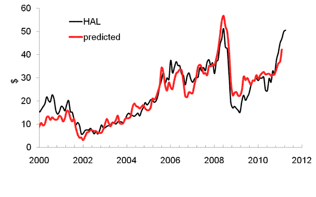
HAL = -3.5dCPI(t-1/6) + 43; 1999-2009

Figure 1. The observed and predicted share prices.

Figure 1 displays all five models with coefficients obtained in 2009. All in all, the prediction was excellent and these prices are likely defined by the difference between the core CPI and the headline CPI. Considering increasing oil price, the rise in the share prices is not surprising. When oil price is down, the share will fall.

Kitov, I. (2009). Predicting ConocoPhillips and Exxon Mobil stock price, Journal of Applied Research in Finance, Spiru Haret University, Faculty of Financial Management and Accounting Craiova, vol. I(2(2)_ Wint), pp. 129-134.

Kitov, I., Kitov, O. (2008). Long-Term Linear Trends In Consumer Price Indices, Journal of Applied Economic Sciences, Spiru Haret University, Faculty of Financial Management and Accounting Craiova, vol. 3(2(4)_Summ), pp. 101-112.

Kitov, I., Kitov, O. (2009a). A fair price for motor fuel in the United States, MPRA Paper 15039, University Library of Munich, Germany,

Kitov, I., Kitov, O. (2009b). Sustainable trends in producer price indices, Journal of Applied Research in Finance, Spiru Haret University, Faculty of Financial Management and Accounting Craiova, vol. I(1(1)_ Summ), pp. 43-51.

Kitov, I., Kitov, O. (2009c). Predicting share price of energy companies: June-September 2009, MPRA Paper 15863, University Library of Munich, Germany

Share price modeling for Harley-Davidson

Scientific literature definitely has a positive bias with successful examples more often published than failures. We also add to this bias selecting only successful models. But it is always a pleasure to describe a very stable and accurate model. Harley-Davidson (HOG) is one of the best illustrations of our concept linking stock prices to CPI components. Here we present two models for HOG (see a brief description of the concept in Appendix). One was obtained in September 2009 and covered the period from October 2008. The most recent HOG model uses the monthly closing price for March 2001 and the CPI estimates published on April 14, 2011. (Through 2010, the model was the same as in 2011.)

The importance of the HOG model for our concept is obvious – it validates deterministic character of stock pricing. For investors, it is also important to have a long-term reliable prediction of stock prices.

For HOG, the defining indices are as follows: the index of rent of primary residence (RPR) and the index of owners' equivalent rent of residence (ORPR). Both CPI components are leading the share price. Figure 1 depicts the evolution of the indices which provide the best fit model, i.e. the lowermost RMS residual error, between July 2008 and March 2011. The models are as follows:

HOG(t) = -13.82RPR(t-3) +12.77ORPR(t-4) +17.82(t-1990) – 163.94, before September 2009

HOG(t) = -11.30RPR(t-3) + 9.83ORPR(t-3) +17.53(t-1990) – 36.34, after September 2009

where HOG(t) is the share price in US dollars, t is calendar time.

Both models are depicted in Figure 2. The predicted curves lead the observed ones by 3 months. The residual error is of $4.10 for the period between July 2003 and March 2011. In the second quarter of 2011, the model foresees a fall to the level of $30 per share.

Figure 1. Evolution of the price indices ORPR and RPR.

Figure 2. Observed and predicted POM share prices. Upper panel – the model for September 2009. Lower panel – the model for march 2011.

Appendix

In its general form, our pricing model is as follows:

sp(t_j) = Σb_i∙CPI_i(t_j-t_i) + c∙(t_j-2000 ) + d + e_j (1)

where sp(t_j) is the share price at discrete (calendar) times t_j, j=1,…,J; CPI_i(t_j-t_i) is the i-th component of the CPI with the time lag t_i, i=1,..,I; b_i, c and d are empirical coefficients of the linear and constant term; e_j is the residual error, which statistical properties have to be scrutinized. By definition, the bets-fit model minimizes the RMS residual error. The time lags are expected because of the delay between the change in one price (stock or goods and services) and the reaction of related prices. It is a fundamental feature of the model that the lags in (1) may be both negative and positive. In this study, we limit the largest lag to eleven months. Apparently, this is an artificial limitation and might be changed in a more elaborated model.

System (1) contains J equations for I+2 coefficients. For POM we use a time series from July 2003 to March 2011, i.e. 94 monthly readings. Due to the negative effects of a larger set of defining CPI components their number for all models is (I=) 2. To resolve the system, we use standard methods of matrix inversion. As a rule, solutions of (1) are stable with all coefficients far from zero. In the POM model, we use 92 CPI components. They are not seasonally adjusted indices and were retrieved from the database provided by the Bureau of Labor Statistics.

4/21/11

Pepco Holdings to rise

In this post, we introduce a new model for a company in the energy S&P 500 subcategory – Pepco Holdings (POM). The importance of any energy related company is dictated by the influence of growing energy price on the overall economic performance. For many companies presented in this blog during the past week the forecast for the second quarter of 2011 is not promising. But before presenting the model we would like to refresh the overall approach.

In its general form, our pricing model is as follows:

sp(t_j) = Σb_i∙CPI_i(t_j-t_i) + c∙(t_j-2000 ) + d + e_j (1)

Due to obvious reasons, longer time series guarantee a better resolution between defining CPIs. In general, there are two sources of uncertainty associated with the difference between observed and predicted prices. First, we have taken the monthly close prices (adjusted for splits and dividends) from a large number of recorded prices: monthly and daily open, close, high, and low prices, their combinations as well as averaged prices. Second source of uncertainty is related to all kinds of measurement errors and intrinsic stochastic properties of the CPI and its components. One should also bear in mind all uncertainties associated with the CPI definition based on a fixed basket of goods and services, which prices are tracked in few selected places. Such measurement errors are directly mapped into the model residual errors. Both uncertainties, as related to stocks and CPI, also fluctuate from month to month.

For POM, the defining indices are as follows: the index of food away from home (SEFV) and the index of owners' equivalent rent of residence (ORPR). The CPI components are leading by 4 and 5 months, respectively. Figure 1 depicts the evolution of both indices which provide the best fit model, i.e. the lowermost RMS residual error, between July 2010 and March 2011:

POM(t) = -2.66SEVF(t-4) +1.06ORPR(t-5) +11.83(t-1990) + 101.35

where POM(t) is the share price in US dollars, t is calendar time.

The predicted curve in Figure 2 leads the observed one by 4 months. The residual error is of $0.95 for the period between July 2003 and March 2011. In the second quarter of 2011, the model foresees a rise by $1.5.

Figure 1. Evolution of the price indices ORPR and SEVF.

Figure 2. Observed and predicted POM share prices.

Procter and Gamble - no change in 2011Q2

In July 2010, we presented a model for Procter and Gamble (PG) which forecasted a period of growth from $59 in June (had fell from $62 in March 2010) to $63 in September 2010. This model was defined by the index of food away from home (SEFV - CUUS0000SEFV) and that of rent of primary residency (RPR). The former CPI component led the share price by 3 months and the latter one led by 8 months. The prediction was right and the price reached $63.

For the past ten months, this model is also applicable with only change in the time lead for the SEFV – it is now 4 months. Overall, the model predicted a no change period. Figure 1 depicts the overall evolution of both involved indices since 2003. Considering the fact that the original model was valid for the period since September 2009, these two defining components have been providing the best fit model between August 2009 and March 2011. Relevant coefficients are negative and positive, respectively. The slope of time trend is also positive. So, the best-fit 2-C model for PG(t) is as follows:

PG(t) = -5.4SEFV(t-4) + 2.93RPR(t-8) + 18.16(t-1990) + 187.47

where PG(t) is the monthly closing price (dividend and split adjusted) in US dollars, t is calendar time.

The predicted curve in Figure 2 leads the observed price by 4 months with the residual error of $2.14 for the period between July 2003 and March 2011. In other words, the price of a PG share is completely defined by the behaviour of these two CPI components.

The model does predict the share price in the past and foresees the period of no growth to be extended into the second quarter of 2011.

Figure 1. Evolution of the price of SEFV and RPR.

Figure 2. Observed and predicted PG share prices.

Rise in the price of food. How long yet?

We continue reporting on the evolution of the difference between core CPI and the index for food (beverages not included). In the previous post we confirmed that this difference had been following the long-term (negative) quasi-linear trend since 2001. The main question is when the difference will reach its bottom value and the trend will turn to a positive one. This pivot will manifest the change from increasing to decreasing food price. The importance of this event cannot be underestimated in the current political and economic situation in developing countries, where populations are literally starving.

Previously, we suggested that the remarkable rally in food prices had forced the index for food to grow faster than predicted and the deviation from the trend predicted in 2007 reached ~7 units in 2008 [1]. Originally, the predicted difference (red line in Figure 1) intersected the zero line around 2014.

In January 2009, the trend line was much steeper and crossed the zero line. In March 2011, the (black line) trend crosses the zero line in the end of 2010. Therefore, Figure 1 demonstrates that the difference between the core CPI and the index of food has been slowly approaching to its original trend (red line) since 2009.

Here we suggest that the intercept with the zero line and the pivot to the decreasing food price now seems to start in 2011-2012. The previous negative/positive pivot was at the level of -10, as displayed in Figure 2. If it is the case for the current situation the negative trend will change only in after 2016.

Figure 1. The difference between the core CPI and the price index of food. The pivot point to a positive trend in likely in 2011 or 2012.

Figure 2. The difference between the core CPI and the price index of food between 1960 and 2011.

References

1. Kitov, I., Kitov, O., (2008). Long-Term Linear Trends In Consumer Price Indices, Journal of Applied Economic Sciences, Spiru Haret University, Faculty of Financial Management and Accounting Craiova, vol. 3(2(4)_Summ), pp. 101-112.