Modeling S&P 500 returns. March 2011

We restart (or continue) reporting on the evolution of the S&P 500 and our prediction made in the beginning of 2009. Between March 2009 and September 2010, the prediction based on the number of nine-year-olds, N9, fitted the observed S&P 500 with minor deviations. All in all, sixteen months in a raw we were right and did not see any source which might disturb our prediction. However, there is one source of problem for many economic and econometric models we have built – population distributions provided by the US Census Bureau.

Here, we reintroduce the original model which links the S&P 500 annual returns, Rp(t), to the number of nine-year-olds, N9. To obtain a prediction we use the number of three-year-olds, N3, as a proxy to N9 at a six-year horizon:

Rp(t+6) = 100dlnN3(t) - 0.23 (1)

where Rp(t+6)is the S&P 500 return at a six-year horizon. Figure 1 depicts relevant S&P 500 returns, both actual one and that predicted by relationship (1). The latter curve has been deviating the latter one since October 2010. Currently, this deviation is very big and put our model under strong doubt.

Figure 1. Observed and predicted S&P 500 returns.

This is not the end of the model, however. We continue using the link between real GDP and N9, as described in this paper. It was shown that one can exchange them when one of these two is not well estimated (usually N9). In that sense, one can use real GDP instead on N9.

As discussed in our working paper on S&P 500, there exists a trade-off between the growth rate of real GDP, G(t), and the S&P 500 returns, R(t). The predicted returns, Rp(t), can be obtained from the following relationship:

Rp(t) = 0.0062dlnG(t) - 0.01 (2)

where G(t) is represented by the Q/Q (annualized) growth rate, because only quarterly readings of real GDP are published by the BEA.

With a small correction of the coefficients in (2), Figure 2 displays the observed S&P 500 returns and those obtained using real GDP, as presented by the US Bureau of Economic Analysis. As before, the observed returns are MA(12) of the monthly returns. The period after 2003 is relatively well predicted, including that not predicted by (1). Therefore, it is reasonable to assume that G(t) can be used for modeling of the S&P 500 index and returns. Reciprocally, current S&P 500 may be used for the estimation of real GDP.

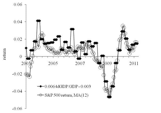
Figure 2. Observed S&P 500 return and that predicted from real GDP. For a given quarter, all monthly values of the growth rate relative to the previous quarter are equal.

To understand the deviation associated with N9 we are waiting for the final results of the 2010 census. This is also crucial for many economic models we have developed for the U.S. Other developed countries do not demonstrate such big deviations.

Inflation and unemployment in Switzerland: from 1970 to 2050

We have started writing a new monograph. As always, it’s an exciting process. This time we would like to collect all results on inflation and unemployment in OECD countries and to carry out a rigorous statistical analysis. We include only those OECD members who provide an extensive statistics on inflation, unemployment and labor force. As a result, some countries will not be modeled.

Switzerland was not fully modeled in our monograph on mechanomics. We have written a paper and submitted it to the MPRA. Now it is available via RePEc:


Inflation and unemployment in Switzerland: from 1970 to 2050
Abstract

An empirical model is presented linking inflation and unemployment rate to the change in the level of labour force in Switzerland. The involved variables are found to be cointegrated and we estimate lagged linear deterministic relationships using the method of cumulative curves, a simplified version of the 1D Boundary Elements Method. The model yields very accurate predictions of the inflation rate on a three year horizon. The results are coherent with the models estimated previously for the US, Japan, France and other developed countries and provide additional validation of our quantitative framework based solely on labour force. Finally, given the importance of inflation forecasts for the Swiss monetary policy, we present a prediction extended into 2050 based on official projections of the labour force level.

Theoretical and Practical Research in Economic Fields: Winter Issue

I am happy to inform all readers that the winter issue of the TPREF is now available.

Table of contents:

Macroeconomic Fundamentals and Stock Return Dynamics: International Evidence from the Global Finance Area

Ezzeddine Abaoub, University of 7 November at Carthage
Mongi Arfaoui,  University El Manar
Hammadi Sliti,  University El Manar ... 122

Financial Integration in the four Basins: A Quantitative Comparison
Sergio Alessandrini,  University of Modena and Reggio Emilia … 147

The Law of One Price: Survey of a Failure
Alessio Emanuele Biondo, University of Catania … 168
The Yield Curve and the Prediction on the Business Cycle: A VAR Analysis for the European Union
Giuseppe Cinquegrana ISTAT, Italy
Domenico Sarno, Department of Law and Economics Second University of Naples … 183

Neuroeconomics and Decision Making Process
Mădălina Constantinescu, Spiru Haret University … 210

Differential Games in Non–Renewable Resources Extraction
George E. Halkos, University of Thessaly
George Papageorgiou, University of Thessaly … 219

Consumption in Developed and Emerging Economies
Peter Kadish, Norvik Alternative Investments … 231

Intelligent Agent Approach for Business Process Management
Andy Ştefănescu, University of Craiova … 241

The Australian Phillips curve and more

This blog helps us to voice new ideas before they are formalized in an article or working paper. In many cases, original ideas are partially wrong and mathematics has to be changed severely. This was the case with labour force participation rate and productivity. As a rule, our initial ideas are good enough and do not suffer big changes.

In January 2011, we posted on inflation and unemployment in Australia. Meanwhile we prepared a formal working paper and submitted it to www.arXiv.org and MPRA. The major difference with the blog posts is a complete description of all models and thorough statistical assessment which includes successful tests for cointegration. However, it needs slight polish before we send it to a journal.

Now the paper on Australia is available:

Abstract

A quantitative model is presented linking the rate of inflation and unemployment to the change in the level of labor force. The link between the involved variables is a linear one with all coefficients of individual and generalized models obtained empirically. To achieve the best fit between measured and predicted time series cumulative curves are used as a simplified version of the 1-D boundary elements method. All models for Australia are similar to those obtained for the US, France, Japan and other developed countries and thus validate the concept and related quantitative model.

On real GDP growth in the US

The U.S. Bureau of Economic Analysis (http://www.bea.gov) has reported an estimate of real GDP in the fourth quarter of 2010. Accordingly, a new estimate of the growth rate in 2010 is available. It looks not so bad: +2.9% per year. Let’s ignore the rates of growth for a while and find out where the U.S. stays in terms of real GDP level. Below is a table with quarterly real (in billions of chained 2005 US dollars) GDP estimates since 2007:


2007q1 13,089.3
2007q2 13,194.1
2007q3 13,268.5
2007q4 13,363.5
2008q1 13,339.2
2008q2 13,359.0
2008q3 13,223.5
2008q4 12,993.7
2009q1 12,832.6
2009q2 12,810.0
2009q3 12,860.8
2009q4 13,019.0
2010q1 13,138.8
2010q2 13,194.9
2010q3 13,278.5
2010q4 13,382.6

Well, the US has finally overcome by a 19 billion margin the level of 2007q4. At a healthy pace of 2.5% per year, the rise since 2007 should be around 1 trillion. Moreover, approximately 1% of real economic growth in the U.S. is associated with the overall population increase by 1% per year. In the fourth quarter of 2007, real GDP per capita was $44.292 (civilian population in December 2007 - 301,710,949) and in the same quarter of 2010 - only $43.255. The overall decrease in real GDP per capita since 2007 is 2.3%.

Autodesk stock price to rise in 2011Q1

When modeling stock prices by decomposition into two CPI components and linear time trend we exercise two different  time periods: after January 1994 and after June 2003. The reason for this separation is simple – the difference between individual CPI components is usually characterized by the presence of several linear trends. When linear trend in the difference between two defining CPI components has a pivot point relevant stock model also has a break in all coefficients. Therefore, we usually prefer to avoid this type of bias and limit our modeling to the period after June 2003 when all turns in many CPI difference did happen after the 2001 recession. This shorter modeling period significantly influences the resolution of the model and we would prefer to use longer time series when possible.

The model for Autodesk (ADSK) is an excellent example of the possibility to extend the modeling period back to 1994. The resulting model has a deterministic character and predicts the share price evolution at a several month horizon. Our model for ADSK is stable over the past year and is defined by expected indices: the consumer price index of motor vehicle maintenance and repair (MVR) and the index of information technology, hardware and software (IT). The latter defining index definitely has tight relations to ADSK.

The MVR index leads the share price by 5 months and the IT one - by 8 months. Figure 1 depicts the overall evolution of the difference between the involved indices. As discussed above, no change in the trend has been observed since 1994. Hence, the final share price model for ADSK should not be biased by the change in the trend.

These two defining CPI components provide the best fit model between June 2010 and December 2010. The MVR coefficient is negative and thus the increasing price of motor vehicle maintenance and repair causes the share price to fall. The IT index has a positive coefficient but the long-term decrease in this index also causes the share to fall. The slope of time trend is positive revealing the price tendency to increase over time. The best-fit 2-C model for an ADSK(t) share price is as follows:

ADSK(t) = -3.97MVR(t-5) + 2.18IT(t-8) + 35.25(t-1990) + 265.90

where t is calendar time.

The predicted and observed curves are presented in Figure 2. The residual error is $4.75 for the period between January 1994 and December 2010. The model provides a relatively good prediction of the share price in the past. Currently, the predicted price shows a strong tendency to rise. One should expect the ADSK price to grow fast in the first quarter of 2011.

Figure 1. Evolution of the difference between MVR and IT. No change in the long-term sustainable linear trend is observed.

Figure 2. Observed and predicted ADSK share prices.

Unemployment in Australia

Following the previous post on inflation in Australia, we present a similar model for the rate of  unemployment .

It has been empirically revealed and statistically tested that the rate of unemployment, in developed countries is a linear function of the change in labor force. We expect the same relationship to be valid for Australia. A simple trial-and-error method applied to cumulative unemployment published by the Australian Bureau of Statistics at a monthly rate (see Figure 1) allows to accurately estimating both coefficient in the linear relation:

UE(t) = -2.1dLF(t)/LF(t) + 0.0977; t>1995

UE(t) = -2.1dLF(t)/LF(t) + 0.131; t<1996 (1)

Because of the change in monetary policy around 1995, we had to split the modeled period into two segments: before and after 1995. The above relationships show that only free term did change in 1996 from +0.131 to +0.099. The slope in the linear relationship is the same over the entire period. All in all, the agreement between the annual and cumulative curves is excellent. One can predict the rate of unemployment at any time horizon using labor force projections. We have failed to find any projection published by the Australian Bureau of Statistics except the one between 1999 and 2016. Unfortunately, this projection was all wrong and heavily underestimated the growth in labor force. It predicted the level of labor force in 2016 at 10,800,000. In December 2010, the level of labor force was 12,132,900. This is good news, however. According to (1), a higher rate of labor force results in a lower rate of unemployment.

Figure 1. Upper panel. Monthly estimates of the rate of unemployment in Australia and that obtained from labor force using (1). Due to high-amplitude fluctuations in the monthly estimates of dLF/LF, the predicted curve is smoothed by a twelve-month moving average, MA(12). Lower panel. Cumulative values of the observed and predicted curves in the upper panel. Notice excellent agreement between the cumulative curves.