Copper ores and grains. A year after

About a year ago we published a prediction for copper and grain:

Therefore, copper price will likely not be growing to its peak in April 2008 (491.7), but will likely return to heights around 350.

In the short-run, the index for copper will be growing at least till the end of 2009. The index for grains will continue its decline relative to the PPI. As a consequence, one can expect that the index for food will be also decreasing and this decline will stretch into the 2010s.

Figure 1 compares the prediction and actual behavior for the producer price index of copper ores relative to the overall PPI. All in all, the prediction was right: by the end of 20009 the price index of copper has reached the level of 350 (375) and even higher in the beginning of 2010 (443 in April). However, it has not reached the 2008 level. It is difficult to foresee further evolution, but one cannot exclude the price to grow beyond that in 2008.

Figure 2 illustrates the accuracy of our prediction of the index of grains. The index has been falling relative to the PPI and the trajectory actually repeats that observed 142 months before, as explained the previous post:

It is instructive to compare two major spikes in the grains index in 1996 and 2008 relative to the PPI. In order to avoid comparing absolute values, which undergo secular growth, the evolution of the difference between the PPI and the price index of grains normalized to the PPI. Figure 3 presents the normalized curves. The left panel shows that the spike in the grains PPI in July 1996 is similar in relative terms to that observed in 2008. The right panel tests this hypothesis: the spikes are synchronized - for the black line is shifted forward by 142 months. From this comparison, it is likely that decline in the grains index relative to the PPI will extend into the 2010s.

Figure 1. Evolution of the price index of copper ores relative to the PPI. Upper panel: September 2009. Lower panel: April 2010.

Figure 2. Evolution of the difference between the PPI and the price index of grains normalized to the PPI. Left panel: September 2009. Right panel: April 2010.

Short term prediction

In the short-run, the index for copper will NOT be growing too long, at least NOT till the end of 2010. The index for grains will continue its decline relative to the PPI. As a consequence, one can expect that the index for food will be also decreasing and this decline will stretch into the 2011.

We can also repeat the conclusion from the post one year ago

In the long run, the producer price index for copper and that of grains both demonstrate practically unpredictable behavior with unclear future. This observation only emphasizes the importance of sustainable trends observed for other commodities. In the US economy, as in many natural systems, there exist trend components, oscillating components, and random components.

PPI of metals: annual revision

About a year ago we revised the evolution of several price indices of metals. Our general approach is based on the presence of long-term sustainable trends in the evolution of the CPI and PPI in the United States. The difference between various components of these indices is not a random but rather a predetermined process, as shown in a series of papers we published in 2008-2009 [1-4]. Using these trends, one can predict consumer and producer price indices for select goods, services and commodities [5-7]. We have summarized these papers and some more studies in a monograph “Deterministic mechanics of pricing” published by LAP [8].

In this post, we revisit the trends in the PPI of three commodities related to metals: steel iron, nonferrous metals, and metal containers. Originally, these items were studied in our article [4]. This is a regular revision with the next scheduled to the end of 2010.

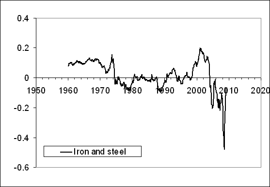
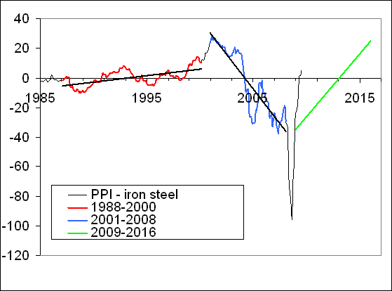
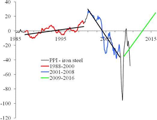
1. Figure 1 compares the original (upper panel), revised (middle panel) and the newly updated differences. According to [4]:
“the normalized difference between the PPI and the index for iron and steel (101) is characterized by the presence of a sharp decline between 2001 and 2008: from +0.2 to -0.4. Between 1980 and 2000, the curve fluctuates around the zero line, i.e. there was no linear trend in the absolute difference. One could expect the negative trend is now transforming into a positive one.“

A year ago we wrote:
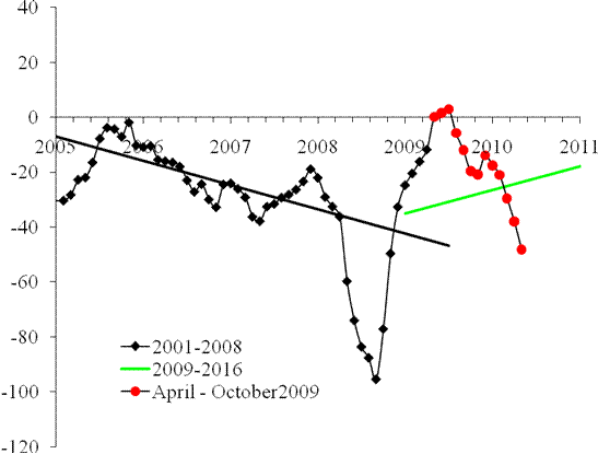
“Between March and June 2009, the difference continued to increase, and likely reached its peak in June (Figure 2). In July or August 2009, the difference will stall around its peak value and then will start to decrease. As a result, the index for iron and steel will be growing faster than the PPI. In the short run, one can expect a fast recovery of iron and steel prices to the level observed in January-March 2008, i.e. the index will reach the level 210 to 220. However, this recovery will not stretch into 2011, and the index of iron and steel will be declining in the long run to the level of 2001, as depicted in Figure 3. In other words, the period between 2008 and 2010 is characterized by very high volatility, which will fade away after 2011. “

This prediction was right, as Figures 2 and 3 in this post demonstrate.

2. According to [4]:
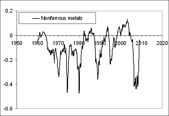
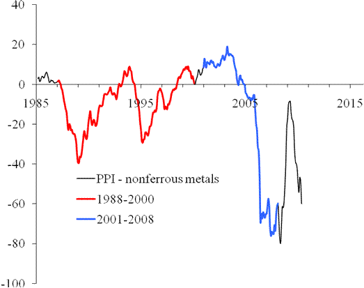
“the index for non-ferrous metals (102) shows an example of the absence of sustainable trends in the normalized difference. The curve is rather a comb with teeth of varying width. Although varying, the distance between consecutive troughs is several years at least. Therefore, one should not expect a quick recovery in the price for nonferrous metals”.

A year ago we wrote:
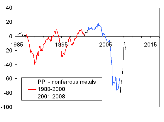
Figure 4 displays the original and updated predictions. There is almost nothing to add to the previous statement. The recovery in March-June 2009 is likely only a short-term one, as the past experience shows.

We also display in Figure 4 the newly updated trajectory. As forecasted, the producer price index of nonferrous metals has regained its price setting power, and the March-June 2009 excursion in the difference was only temporary. It should not last long, however.


3. It was stated in [4] that,
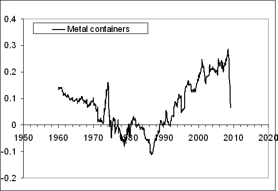
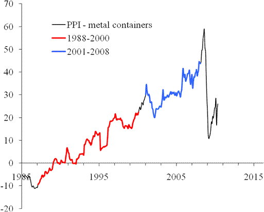
“the index for metal containers (103) provides an excellent example of linear trends in the normalized difference. There are two distinct periods between 1960 and 2008 with a turning point in 1987. A sudden drop in the difference in the end of 2008 may symbolize the start of transition to a new period with a negative trend. Then the price for metal containers will be increasing at an elevated rate, i.e. the index will get back its price setting power.”

A year ago we wrote:
Figure 5 presents the original and updated versions of the difference between the PPI and the index of metal containers. The negative overshoot in the difference reached its peak in March and currently the difference started to increase. One can not exclude short-period oscillations in the near future. The future of the index for metal containers is vague.

The difference was on an upward trend since June 2009 with a short-period fluctuation, as expected. The evolution along the positive trend should continue into 2011, i.e. the price index of metal containers will be losing its pricing power relative to the overall PPI.


Conclusion
Our simple predictions were good enough and validate the general concept of the sustainable trends in the CPI and PPI differences. Will keep reporting on the further developments.




Figure 1. Upper panel: The evolution of the difference between the PPI and the price index of iron and steel between July 1985 and March 2009 (borrowed from [4]). Middle panel: Same for the period between 1985 and June 2009. Red and blue lines highlight segments between 1988 and 2001, and from 2001 to 2008, respectively. Green line predicts the evolution of the difference after 2008, as a mirror reflection of the linear trend between 2001 and 2008. Lower panel: The difference updated for the period between June 2009 and April 2010. As expected, the difference has been decreasing during the reported period and sank below the new trend (green). The trajectory has to turn up in the near future and reach the new trend by July 2011. This means that the price index for iron and steel will be growing at a lower rate than the overall PPI.



Figure 2. Upper panel: The evolution of the difference between the PPI and the price index of iron and steel between January 2005 and June 2009. Red line predicts the evolution of the difference after 2008. Red circles represent the difference between April and June 2009. We expect the difference will start growing in August-September 2009. Lower panel: The newly updated trajectory. The difference precisely obeyed our prediction a year ago and sank below the green line (new trend).



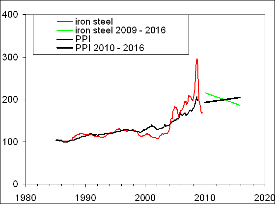
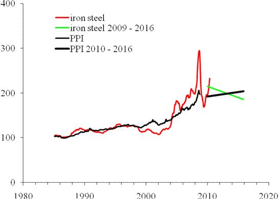
Figure 3. Upper panel: The evolution of the PPI, the index for iron and steel, and their difference in the long-run between 2009 and 2016. The index for iron and steel is predicted to decrease from the level of 220, which it will reach by the end of 2009, to ~185 in 2016. Accordingly, the difference will be growing as shown in Figure 1. The PPI will be also slowly growing. Lower panel: The newly updated trajectory.






Figure 4. Upper panel: The evolution of the difference between the PPI and the index of nonferrous metals from 1960 to March 2009 (borrowed from [4]). Middle panel: Same as in the upper panel for the period between 1985 and June 2009. There are no linear trends in the difference, but its behavior demonstrates a clear periodic structure with relatively deep but short troughs, which reflect the fast growth in the PPI for nonferrous metals. The last excursion ended in 2009. A period of hovering near the zero line is expected. Lower panel: The newly updated trajectory. As forecasted, the producer price index of nonferrous metals has regained its price setting power, and the March-June 2009 excursion in the difference was only temporary. It should not last long, however.




Figure 5. Upper panel: The evolution of the difference between the PPI and the index of metal containers from 1960 to March 2009 (borrowed from [4]). Middle panel: Same as in the upper panel for the period between 1985 and June 2009. There are distinct linear trends in the difference. One can not exclude that the fall in the difference is a start of the transition to a new trend. Lower panel: The newly updated trajectory.


References

1. Kitov, I., Kitov, O., (2008). Long-Term Linear Trends In Consumer Price Indices, Journal of Applied Economic Sciences, Spiru Haret University, Faculty of Financial Management and Accounting Craiova, vol. 3(2(4)_Summ), pp. 101-112.
2. Kitov, I., (2009). Apples and oranges: relative growth rate of consumer price indices, MPRA Paper 13587, University Library of Munich, Germany.
3. Kitov, I., Kitov, O., (2009). A fair price for motor fuel in the United States, MPRA Paper 15039, University Library of Munich, Germany,
4. Kitov, I., Kitov, O., (2009). Sustainable trends in producer price indices, Journal of Applied Research in Finance, v. 1, issue 1.
5. Kitov, I., Kitov, O., (2009). PPI of durable and nondurable goods: 1985-2016, MPRA Paper 15874, University Library of Munich, Germany
6. Kitov, I., (2009). Predicting gold ores price, MPRA Paper 15873, University Library of Munich, Germany
7. Kitov, I., (2009). Predicting the price index for jewelry and jewelry products: 2009-2016, MPRA Paper 15875, University Library of Munich, Germany
8. Kitov, I. (2010). Deterministic mechanics of pricing. LAP Academic Publishing, Saarbrucken, Germany.

CPI and core CPI. Two years later

Two years ago we published a paper on the presence of long-term sustainable trends in the differences between various components of the CPI in the USA. We started with the difference between core CPI (i.e. CPI less food and energy) and overall CPI. Two Figures below are borrowed from the paper Figure 1. Linear regression of the difference between the core CPI and CPI for the period from 1981 to 1999. The goodness-of-fit is 0.96, and the slope is 0.67.

Figure 2. Linear regression of the difference between the core CPI and CPI after 2002. The goodness-of-fit is 0.86, and the tangent is -1.57. An elevated volatility has been observed from 2005.

We also suggested in this and later papers on the sustainable trends in the CPI and PPI (see here) that the negative trend shown in Figure 2 should reach some bottom point and turn to a positive trend. It was also mentioned that such processes in the past had been accompanied by an elevated volatility in the difference, i.e. high amplitude fluctuations.

Now, two years later, we plot the difference again and are happy to conclude that our prediction has realized in practice. We announce the beginning of the positive trend, as Figure 3 shows. The trend should be observed at least five to eight years and will be characterized by a faster growth in prices of goods and services not associated with food and energy. We will keep posting on the difference.

Same pivot is observed in many other, but not all(!), differences mentioned in the original paper.

Figure 3. A positive trend has been emerging since December 2010. The differnce will likely grow from 3 in the beginning of 2010 to 11 in 2016. Accordingly, energy and food will lose their pricing power relative to the core CPI goods and services.

Crude price in August 2010

A month ago we presented a forecast for oil price. It’s time to revisit the price. All our estimates are based on the existence of long-term sustainable trends in the differences between various subcategories of the producer price index (PPI). The concept and numerous forecasts is published in this paper. The dry residual is that the producer price indices evolve along straight lines, with all deviations from the trend cancelling themselves out over relatively short periods of several months.

Figure 1 present the case of crude petroleum (domestic production) for the period between 2007 and 2012. We have predicted that the difference between the overall PPI and the index for oil will be on a upward trend since 2009. This means than the PPI will grow faster than the index of oil, the latter likely to fall into 2016 down to the level of ~75.

In March and April 2010, the index of crude petroleum had a bigger deviation out of the trend in Figure 1. Therefore, the most likely next movement in the price will be the return to the trend. Moreover, the difference will likely to break the trend line and go into the other side for several months. This would mean the price of oil falling in May 2010 and during the summer months, as shown in Figure 1 by red circles. Tentatively, we put the index at the level between 160 and 180 in August 2010. Relevant crude oil price will be between $62 and $70 per barrel.

Figure 1. The difference between the overall PPI and the index for crude petroleum. The new predicted trend is shown by dashed line. In May and likely in summer 2010, the index for oil will be decreasing. The difference will be growing as shown by red circles.

P.S. Apparently, oil price lost several dollars in May 2010, and one could say that this post is a bit late and just declares known facts. This is the Bureau of Labor Statistics who reports the PPI and its components in the middle of the next month. Our concept would fail to predict that this is exactly May 2010 when oil price should stop to grow. However, the currently observed level of price is not viable. The price must fall at some point, the larger is the deviation the faster and more violent is the recovery.

S&P 500 in June 2010

As has already been discussed many times since March 2009 and also documeted in a working paper (S&P 500 returns revisited), we expect the S&P 500 stock market index to be gradually decreasing at an avearge rate of 46 points per month. In this post on S&P 500 (01/05/2010), we put the closing level of S&P 500 in May 2010 at 1132 (miscalculation, should be 1142). The actual closing level was 1090 (-97 relative to April 2010), i.e. 42 points below the predicted one. One could expect that kind dynamic "overshoot" in the beginning of a new trend. Same purely emotional effect was observed in March (+69) and April 2009 (+74), when the S&P 500 was increasing much faster than the average rate for the whole period of the rally between March 2009 and April 2010.

So, one might not exclude that the panic of May 2010 will last another month and the closing level of S&P 500 in June will be below 1095, as would be predicted by the rate of -46 points per month starting with 1187 in April 2010. By the end of the summer, the fall will likely decelerate. But the overall downward trend will continue and extend into 2011.

Russian language

Russian was a popular language a century ago. All in all, it was due to great writers and revolutionary movements. Now it loses its popularity worldwide. The reason is obvious - there is nothing interesting Russia can offer to the broader international community. No intellectual breakthrough or/and social process of importance for people as a solution to their own problems.
So, the portion of the world's population speaking or understanding Russian decreases over time. After the disintegration of the Soviet Union - at a dramatically high rate. The question is : What to do?
There are two points of potential improvement. We need to make ourselves to be interested in ... ourselves focusing on the fact that, with all these external changes, we retain the core of our souls, which was inherited from the generations before us. At the same time, the transition to the new social construction allowed us to aquire in a very short time what other nations have been accruing during the past century. As a benefit, we could avoid all mistakes already made.
Such an analysis would be instructive for everybidy.

Deterministic share prices

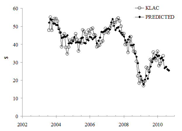
Here we display a number of models with predictable future prices. The models are listed below and their predictions are compared with actual observations in a series of relevant figures.

Table 1. The best fit 2C models

AAPL(t)= 19.031HFO(t-13) - 10.134HOS(t- 0) + 73.864(t-1990) - 1862.561, stdev=$13.76
ADSK(t)= -3.725RPR(t-12) - 2.8 HOS(t-1) + 42.307(t-1990) + 613.209, stdev=$3.36
AMAT(t)=-2.89SEFV(t-2) + 2.212RPR(t-7) + 2.483(t-1990) + 61.366, stdev=$1.23
AMGN(t)=0.903DIARY(t-13) - 4.705AB(t-0 ) + 18.687(t-1990) + 539.676, stdev=$4.11
ANF(t)=-3.761OFH(t-1) - 2.764TS(t-5) + 34.937(t-1990) + 752.703, stdev=$5.43
ASH(t)=-8.575SEFV(t-2) - 2.294MISS(t-5) + 83.36(t-1990) + 1090.622. stdev=$3.71
BDX(t)=-1.785OFH(t-1) + 2.182MISS(t-0) - 8.053(t-1990) - 185.45, stdev=$3.09
BMS(t)=0.597PDRUG(t-6) - 2.108CE(t-5) + 4.599(t-1990) + 163.86, stdev=$1.35
BMY(t)=-0.285DIARY(t-6) - 0.449ITR(t-2) + 5.911(t-1990) + 75.784, stdev=$1.16
C(t)=-0.898DIARY(t-4) - 6.017SEFV(t-11) + 38.966(t-1990) + 729.119, stdev=$2.6
CHK(t)=-1.003OFH(t-3) + 0.274E(t-0) + 4.117(t-1990)+ 78.411, stdev=$3.74
COH(t)=-4.651RPR(t-0) - 20.295IT(t-0) + 15.027(t-1990) + 1085.555, stdev=$2.85
CPB(t)=-1.463SEFV(t-5)+1.04MCC(t-7)+4.667(t-1990)-49.405, stdev=$1.19
CSC(t)=-3.766MVP(t-1)+3.203SPO(t-7)+16.105(t-1990)-147.796, stdev=$3.18
CVS(t)=-0.583OFH(t-4)-1.017TS(t-5)+11.392(t-1990)+172.62, stdev=$1.58
DIS(t)=-1.132FH(t-5)-0.638ITR(t-2)+13.33 (t-1990)+168.775, stdev=$1.64
DTE(t)=-1.622HOS(t-0)+1.34MCC(t-8)-0.196(t-1990)-65.675, stdev=$1.59
DYN(t)=-2.098SEFV(t-2)+1.258RPR(t-3)+ 4.945(t-1990)+59.983 , stdev=$0.62
EK(t)=-2.416SEFV(t-6)-1.612SPO(t-0)+14.535(t-1990)+445.406 , stdev=$2.04
EMC(t)=1.499HFO(t-12)-0.935HOS(t-0)+4.61(t-1990)-96.342, stdev=$1.44
EQR(t)=-3.23SEFV(t-3)+1.083PDRUG(t-6)+12.475(t-1990)+84.574, stdev=$2.14
FDX(t)=-11.884SEFV(t-2)-0.949BABY(t-4)+81.188(t-1990)+ 228.808, stdev=$5.46
FITB(t)=-4.883SEFV(t-3)+1.478HOS(t-7)+ 21.354(t-1990)+407.899, stdev=$1.78
GT(t)=-0.258AIRF(t-5)-13.955IT(t-1)-11.986(t-1990)+451.962, stdev=$2.55
HCP(t)=1.364MCC(t-6)+0.27FS (t-0)-8.569(t-1990)-287.318, stdev=$2.05
HOG(t)=-11.195RPR(t-3)+10.379ORPR(t-3)+13.243(t-1990)-119.185, stdev=$3.58
HPQ(t)=-3.155FB(t-5)+2.711RPR(t-6)+4.926(t-1990)-36.904, stdev=$2.06
JNJ(t)=-0.158AIRF(t-7)-2.368PCP(t-3)+7.058(t-1990)+346.745, stdev=$2.34
JWN(t)=-8.525SEFV(t-2)+2.938PCP(t-1)+56.92(t-1990)+330.459, stdev=$2.74
K(t)=-2.394SEFV(t-5)-0.084E (t-7)+20.544(t-1990)+191.489, stdev=$1.7
KLAC(t)=-3.946F(t-4)+3.152RPR(t-5)-1.479(t-1990)+137.268, stdev=$3.6
L(t)=-2.344FB(t-6)-1.687TS(t-4)+28.28(t-1990)+407.023, stdev=$2.11
LCI(t)=1.072MVR(t-11)+0.99DUR(t-13)-8.508(t-1990)-190.04, stdev=$1.02
MAR(t)=-4.548SEFV(t-0)-7.48IT(t-0)+24.214(t-1990)+636.196, stdev=$2.2