The rate of unemployment in the U.S. will fall to 6.2% by 2014

On March 1, 2012 we predicted (in a Seeking Alpha post) the rate of unemployment in the U.S. to fall down to 7.8% by 2013. The BLS announced 7.8% for September 2012. Here we present our basic model and predict the evolution of unemployment in 2013.

In 2006, we developed three individual empirical relationships between the rate of unemployment, u(t), price inflation, p(t), and the change rate of labour force, LF(t), in the United States. We also built a general relationship balancing all three variables simultaneously. Since measurement (including definition) errors in all three variables are independent it may so happen that they cancel each other (destructive interference) and the general relationship might have better statistical properties than the individual ones. For the USA, the best fit model for annual estimates was a follows:

u(t) = p(t-2.5) + 2.5dLF(t-5)/dtLF(t-5) + 0.0585 (1)

where inflation (CPI) leads unemployment by 2.5 years (30 months) and the change in labor force leads by 5 years (60 months). We have already posted on the performance of this model several times.

For the model in this post, we use monthly estimates of the headline CPI, u, and labor force, all reported by the US Bureau of Labor Statistics. The time lags are the same as in (1) but coefficients are different since we use month to month-a-year-ago rates of growth. We have also allowed for changing inflation coefficient. The best fit models for the period after 1978 are as follows:

u(t) = 0.63p(t-2.5) + 2.0dLF(t-5)/dtLF(t-5) + 0.07; between 1978 and 2003

u(t) = 0.90p(t-2.5) + 4.0dLF(t-5)/dtLF(t-5) + 0.30; after 2003

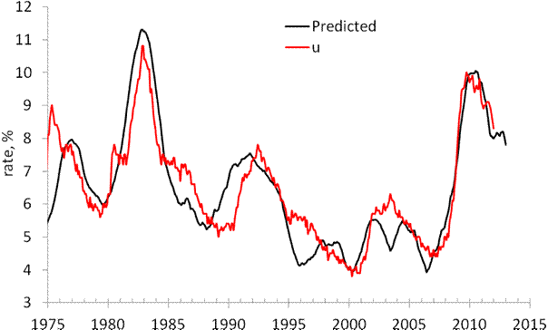
There is a structural break in 2003 which is needed to fit the predictions and observations in Figure 1. Due to strong fluctuations in monthly estimates of labor force and CPI we smoothed the predicted curve with MA(24).

The structural break in 2003 may be associated with the change of sensitivity of the rate of unemployment to the change of inflation and labor force. Alternatively, definitions of all three (or two) variables were revised around 2003, which is the year when new population controls were introduced by the BLS. The Census Bureau also reports major revisions to the Current Population Survey, where the estimates of labor force and unemployment are taken from.

On March 1, 2012 the monthly model predicted a drop from 8.3% in February to 7.8% by the end of 2012. Figure 1 depicts the original prediction (upper panel) and the observed fall in the rate of unemployment (lower panel). Figure 2 shows that the observed and predicted time series are well  correlated (Rsq.=0.81). This is a good statistical support to the model.

Figure 3 depicts the predicted rate of unemployment for the next 12 months. The model shows that the rate will fall to 6.2% by September 2013. For 105 observations since 2003, the modelling error is 0.4% with the precision of unemployment rate measurement of 0.2% (Census Bureau estimates in Technical Paper 66).

 

Hence, one may expect 6.2% [±0.4%].

 

 

Figure 1. Observed and predicted rate of unemployment in the USA as obtained in March and October 2012.

Figure 2.  Observed vs. predicted rate of unemployment between 1967 and 2012. The coefficient of determination   Rsq=0.81.

Figures 3. The predicted rate of unemployment. We expect the rate to fall down to 6.2% in September 2013.

How many democrats are needed to bias unemployment figures?

I do not consider any possibility that the Current Population Survey conducted by the U.S. Census Bureau for September 2012 is biased by CB or by the BLS, This is not the case. There is another hypothetical way to bias the data. There are around 70000 households surveyed by the CB. These households include approximately 200000 persons (mean household is 2.5 people). All these people (excluding several percent not responding ones) answer a few questions associated with their current status: employed, unemployed or not in the labor force. There current level of civilian labor force is approximately 155,000,00 with 12,000,000 unemployed. These figures are calculated by a projection of 200,000 to 310,000,000 using population controls. In essence, one person represents 1550 people.

How many people are needed to increase the rate of unemployment by 0.1%? The rate of unemployment is calculated as the ratio of the number of unemployed and labor force.   So, 0.1% of unemployment rate with the level of labor force of 155,000,000 corresponds to 155000. Since one person in the CPS represents 1550 people, one needs only 100 people to increase the rate of unemployment by 0.1%. To decrease the rate by 0.3% , only 300 (democrats -Spartans?) are needed.

I do not say that the result for September 2012  is biased. I say that the Current Population Survey procedure is wide-open for manipulations.

7.8% unemployment was predicted in April 2012

In 2006, we developed three individual empirical relationships between the rate of unemployment, u(t), price inflation, p(t), and the change rate of labour force, LF(t), in the United States. We also built a general relationship balancing all three variables simultaneously. Since measurement (including definition) errors in all three variables are independent it may so happen that they cancel each other (destructive interference) and the general relationship might have better statistical properties than the individual ones. For the USA, the best fit model for annual estimates is a follows:

u(t) = p(t-2) + 2.5dLF(t-5)/dtLF(t-5) + 0.0585 (1)

where inflation (CPI) leads unemployment by 2 years and the change in labor force by 5 years. We have already posted on the performance of this model several times.

Here a model with monthly estimates of CPI, u, and labor force is presented. The time lags are the same as in (1) but coefficients are different since we use month to month a year ago rates of growth. We have also allowed for changing inflation coefficient. The best fit models for the period after 1978 are as follows:

u(t) = 0.63p(t-2) + 2.0dLF(t-5)/dtLF(t-5) + 0.07; between 1978 and 2003

u(t) = 0.90p(t-2) + 4.0dLF(t-5)/dtLF(t-5) + 0.30; after 2003

There is a structural break in 2003 which is needed to fit the predictions and observations in Figure 1. Due to strong fluctuations in monthly estimates of labor force and CPI we smoothed the predicted curve with MA(24). The rate of unemployment became more sensitive to the change of inflation and labor force. Alternatively, definitions of all three (or two) variables were revised around 2003, which is the year when new population controls were introduced by the BLS.

All in all, the monthly model predicts the observed rate of unemployment which has recently dropped to 8.3%. We expect the rate to fall further to the level of 7.8% by the end of 2012.



Figure 1. Observed and predicted rate of unemployment in the USA.

Unemployment in Spain will be increasing further

Here we revisit the rate of unemployment, ut, in Spain using its dependence on the change in labor force, lt=dLF/LFdt. There is a new estimate of 22.8% for the unemployment rate in 2011. In May 2011, we quantitatively predicted that this rate should only be growing. It may reach 29% if the link between the rate of unemployment and the rate of labor force change is correct, as has been observed since 1980.

Previously, it was found that Spain is characterized by the same relationship between unemployment and labor force as other developed countries. For Spain, we used data provided by the OECD. Figure 1 depicts unemployment and the change rate of labor force between 1960 and 2011. In line with the OECD description of the breaks in the labor force series:

Series breaks: In 2005, changes in the questionnaire and the implementation of CATI system in the field work affected the estimates. The 2005 questionnaire produced an additional increase of employment (132 000) and a decrease of unemployment (78 000). From 2001, the new unemployment definition established by the European Commission in 2000 has been introduced. From 1994, persons employed in the “Guardia Civil” are not included in the armed forces. As an indication, this category represented 59 600 people in 1994. In 1976, the lower age limit for inclusion in the Labour Force Survey was raised from 14 to 16, at the same time other modifications to the survey were introduced.

there are two spikes in the dLF/LF series near 1976 and 2001 as related to step revisions to the level. The spike around 1988 has no explanation in terms of the revisions to labor force, but is of the same amplitude. One can not exclude the opportunity that this spike is related to the processes of joining the EU in 1986.

As expected, the same functional form of dependence is valid for Spain. The estimation method is based on trial-and-error approach and seeks for the fit between annual curves. The final model is as follows

ut = -7.0lt + 0.31; t>1986

Figure 2 depicts observed and predicted curves. Before 1986, the curves diverge and a different model is likely holds. Because of high-amplitude oscillations in the original time series for the rate of labour force change, lt, we have to smooth it by MA(3). For the period after 1986, R2=0.7. Thus, the change in labor force has been driving the rate of unemployment in Spain. The negative coefficient implies that unemployment is Spain goes down when labor force starts to increase.

As has been predicted by our model, the rate of unemployment has increased in 2011. This is not the end of the sad story on unemployment in Spain. Figure 2 evidences that it will likely be growing further with the decreasing labor force.

Figure 1. Unemployment rate, u, and the rate of labor force change, l, in Spain according to the definition introduced by the OECD.

Figure 2. Prediction of inflation by labor force. Due to high variation in the estimates of labor force we have smoothed it with MA(3). For the observed and predicted curves, R2=0.7 for the period between 1986 and 2011.

Why the Economic Projections of Federal Reserve Board are inconsistent

The FRB members have recently projected the evolution of key macroeconomic variables including real GDP and the rate of unemployment. In our blog , we have developed a very accurate model linking the rate of unemployment in the US to the rate of real GDP (per capita) growth: (A series of posts has resulted in a working paper.) The following relationship was estimated:

du = -0.62dlnG + 1.09,  (1)

When integrated between t0 and t, equation (1) can be rewritten in the following form:

u(t) = u(t0) + bln[G/G0] +a(t-t0) + c  (2)

Without loss of generality, we assume t0=0. The intercept c≡0, as is clear for t=t0. Instead of integrating (2), we calculate cumulative sums of the annual estimates of du and lnG with appropriate initial conditions. The cumulative sum of du’s is the time series of the unemployment rate. Figure 1 depicts the measured and observed curves for the period between 1958 and 2011. The agreement is excellent and has been obtained by a formal statistical method (LSQR).

 From (1) it follows that higher rates of GDP growth decrease the rate of unemployment. The FRB has projected real GDP with the highest rates of 2.7% in 2012, 3.2% in 2013, and 4% in 2014. We reduce these rates by 1% per year to estimate the per capita rate of growth, i.e. the growth in population is 1% per year. Using (2) we calculate the rate of uneployment which will correspond to the projected real GDP.

Figure 1 also depicts these predicted rates for 2012 to 2014 by open circles. The rates of unemployment projected by the FRB are shown by red circles. There is a significant deviation between the predicted and projected rates, which likely manifests the inconsistency in the FRB member's models of unemployment.

One may check these projections in 2015. 

Figure 1. The observed and predicted rate of unemployment in the USA between 1958 and 2010.The projected rate of unemployment (middle point of the projections) is shown by red circles. 

Beware of the BEA!

In our previous post, we mentioned a structural break in the Okun’s law around 1978. We explained this break by an artificial change in the definition of the GDP deflator (as defined by the Bureau of Economic Analysis) in the very same time, as also was described in this blog. Here we test quantitatively the change in the estimated Okun’s law coefficients as related to the introduction some new definition of GDP.

Figure 1 displays two time series – the consumer price index, CPI, and the gross domestic purchases price index, dGDP. These time series diverge since 1978 and thus the estimates of real GDP, which is nominal GDP reduced by the GDP deflator, are biased relative to the period before 1978. One should not use the real GDP time series as it is published by the BEA when modelling longer time series including years before and after 1978.

The CPI and dGDP curves coincide when the latter one is corrected by a factor of 1.2, as is also shown in Figure 1. Therefore, one must use the corrected GDP deflator when modelling a time series covering periods before and after 1978.

Figure 1. CPI, dGDP, and 1.2*dGDP.

We made a silly mistake in our study of Okun’s law when tried to use the estimates of real GDP published by the BEA and had to introduce an artificial structural break in order to fit both periods. The best-fit model (Okun’s law) minimizing the RMS error was as follows:

du = -0.406dlnG + 1.113, t<1979

du = -0.465dlnG + 0.866, t>1978

where du is the change in the rate of unemployment and dlnG in the change rate of real GDP per capita. All coefficients we estimated by a LSQ technique minimizing the overall model error. Figure 2 shows the predicted and observed rate of unemployment between 1950 and 2010.

Thus, the structural break expresses itself in a change of slope and intercept around 1978, this year was also estimated in the same LSQ procedure. The ratio of slopes is 1.15, i.e. very close to 1.2 obtained from the CPI and dGDP. Considering the uncertainty in both slopes in the above relationship, which is approximately 0.05, one can conclude that the break in 1978 is entirely artificial and our version of Okun’s law has no structural breaks whatsoever. Essentially, the predicted curve in Figure 2 could be obtained in one piece with a correct dGDP. One has to use the same definition of GDP before and after 1978.

Beware of the BEA! It is not a surprise that economists can not find any clear relationships between macroeconomic variables - they are wrongly measured and misrepresented.

Figure 2. Observed and predicted rate of unemployment in the US.

Some corrections to David Altig's job market charts

David Altig presented some projections of the unemployment rate based on various monthly increments in employment.  It was a crude estimate because it did not include inherent fluctuations in the growth of working age population and labor force participation rate. It is much better to use Okun’s law linking unemployment and the real GDP growth.

Previously in this blog, we presented a version of Okun’s law for the rate of unemployment in the USA since 1955 as defined by real GDP per capita. We have estimated Okun’s law coefficients in two different segments using a standard LSQ technique. The reason behind the split into two segments was the change in realGDP estimation procedure introduced around 1978 - the definition of the GDP deflator was dramatically changed. We discussed this important methodical issuein our blog.

The best-fit (dynamic) model minimizing the RMS error of the cumulative model is as follows:

du = -0.406dlnG + 1.113, t<1979

du = -0.465dlnG + 0.866, t>1978 

This model suggests a smaller shift in the slope and a larger change in the intercept around 1979. This Okun’s law is characterized by a standard error of 0.53% for the period between 1958 and 2010. The average rate of unemployment for the same period is 5.6% with an average annual increment of 1.06%.

            Using the relationship for the period after 1979, one can estimate the evolution of the unemployment rate for various growth rates o real GDP per capita. We have selected three different values: 1% per year, 1.86% per year, and 3% per year. The first value is approximately equal to the mean growth rate between 2000 and 2010 (11 years) which is 0.93% per year. The second value provides a constant rate of unemployment, as defined by the ratio of coefficients 0.866/0.465 and is slightly higher than the mean rate after 1980 (1.63% per year). The third value is very high and just demonstrates the condition to reduce the rate of unemployment to 4% by 2020.  Figure 1 depicts the predicted and observed rate of unemployment after 1980 and these three projections. This is a more accurate projection than that by David Altig.

I do not see any opportunity for the rate of unemployment to fall any time soon. In the long run, unemployment will remain high. For the slow growth scenario expected by the FRB, u may reach 13% by 2020.

 Figure 1. Observed, predicted and projected rate of unemployment in the USA.

Employment in Japan

We continue modeling the evolution of the employment rate in developed countries with Japan. In this study we use the trade-off between the change in unemployment and employment and Okun’s law. Figure 1 compares the change in the rate of employment (the employment/population ratio), de, and the rate of unemployment, du, in Japan. The change in the rate of unemployment is as volatile as that of unemployment and they differ drastically compared to the synchronized evolution of these variables in the U.S. That’s why we have failed to obtain a reasonable Okun’s law for Japan. As before, all data sets on unemployment and employment have been retrieved from the U.S. Bureau of Labor Statistics. The estimates of real GDP per capita have been retrieved from the database provided by the Conference Board.

Figure 1. The (negative) change in the rate of unemployment compared to the change in the rate of employment in Japan.

In this blog, we have already presented several empirical relationships predicting the employment/population ratio from the growth rate of real GDP per capita. This was a natural extension of Okun’s law for unemployment.

Here we estimate an employment/GDP model for Japan similar to Okun’s law. For Japan, the best-fit model has been obtained by the least-squares (applied to the cumulative sums):

det = 0.02dlnGt – 0.53, t<1978

det = 0.14dlnGt – 0.42, t>1977 (1)

 

where dlnGt is the change rate of real GDP per capita at time t. Figure 2 shows the cumulative curves for the time series in (1). There is a structural break near 1978 which is expressed by a dramatic shift in slope and a slight break in intercept. The employment/population ratio varies between from 64%% in 1970 and 56% in 2010. The agreement is excellent. Figure 3 present results of a linear regression with R2=0.95 for the period between 1971 and 2010. We consider both variables as stationary ones over the long run despite the obviously negative trend since 1970.

Figure 2. The cumulative curves for the observed and predicted change in the employment/population ratio, de.

Figure 3. Linear regression of the measured and predicted curves in Figure 2.

Employment in France

There is a trade-off between the change in unemployment and employment. Figure 1 compares the change in the rate of employment (the employment/population ratio), de, and the rate of unemployment, du, in France. As expected, the change in the rate of unemployment is more volatile except the shift in the employment rate near 1982. This is a completely artificial break from 53.2% in 1981 to 55.3% in 1982, and we do not need to model it. All data sets on unemployment and employment have been retrieved from the U.S. Bureau of Labor Statistics.

Figure 1. The (negative) change in the rate of unemployment compared to the change in the rate of employment in France.

In this blog, we have already presented several empirical relationships predicting the employment/population ratio from the growth rate of real GDP per capita. This was a natural extension of Okun’s law for unemployment.

Here we estimate an employment/GDP model for France similar to Okun’s law. For France, the best-fit model has been obtained by the least-squares (applied to the cumulative sums):

de = 0.155dlnG– 0.65, t<1994

de= 0.25dlnG – 0.30, t>1993 (1)

where dlnG is the change rate of real GDP per capita at time t. Figure 2 shows the cumulative curves for the time series in (1). There is a structural break near 1994 which is expressed by significant shifts in slope and intercept. The employment/population ratio varies between from ~56%% in 1970 and 50.4% in 1992. The agreement is very good. Figure 3 present results of a linear regression with R2=0.91 for the period between 1971 and 2010.

Figure 2. The cumulative curves for the observed and predicted change in the employment/population ratio, de.

Figure 3. Linear regression of the measured and predicted curves in Figure 2.

Employment in Canada

There is a trade-off between the change in unemployment and employment. Figure 1 compares the change in the rate of employment (the employment/population ratio), de, and the rate of unemployment, du, in Canada. As expected, the change in the rate of unemployment is more volatile. We have retrieved all data on unemployment and employment from the U.S. Bureau of Labor Statistics.

Figure 1. The (negative) change in the rate of employment compared to the change in the rate of unemployment in Canada.  

In one our previous posts we have estimated Okun’s law for Canada. It is instructive to estimate a model similar to Okun’s law for the employment/population ratio, e. For Canada, the best-fit model has been obtained by the least-squares (applied to the cumulative sums):  

de_t = 0.40dlnG_t – 0.70, t<1984

de_t = 0.56dlnG_t – 0.76, t>1983    (1)  

where dlnG_t is the change rate of real GDP per capita at time t. Figure 2 shows the cumulative curves for the time series in (1). There is a structural break near 1984 which is expressed by a significant shift in slope and a minor change in intercept.  The employment/population ratio varies between from ~54.5% in 1971 and ~64.1% (!) in 2008. The agreement is very good. Figure 3 present results of a linear regression with R²=0.84 for the period between 1971 and 2010.

Figure 2. The cumulative curves for the observed and predicted change in the employment/population ratio, de. 

Figure 3. Linear regression of the measured and predicted curves in Figure 2.

Unemployment in Germany

We have estimated a version of Okun’s law for the USA, France, Spain, Canada, Australia and the UK. We have applied a LSQ technique to the integral version of Okun’s law:  

u(t) = u(t₀) + bln[G/G₀] + a(t-t₀)  (1)  

where u(t) is the predicted rate of unemployment at time t, G is the level of real GDP per capita, a and b are empirical coefficients.  

For Germany, we have estimated a similar model with a structural break somewhere between 1980 and 1990.  The best-fit (dynamic) model minimizing the RMS error of the cumulative model (1) is as follows:

du = -0.32dlnG + 1.19, t<1985

du = -0.43dlnG + 0.81, t≥1985   (2)  

This model suggests a significant increase in slope and a big fall in intercept around 1985.  

Figure 1 depicts the observed and predicted curves of the unemployment rate, the latter is predicted by (1) with coefficients from (2). The agreement is very good, except the years between 2007 and 2009. The deviation is extremely high and unexpected.  During the 2008/2009 recession, the rate of unemployment in Germany was decreasing what contradicts Okun’s law. Our model linking the rate of unemployment to the change in labor force has accurately predicted the observed fall in the unemployment rate.

Figure 2 shows that when the observed time series is regressed against the predicted one, R²=0.86.  Here we do not test both time series for stationarity but presume that the rate of unemployment has to be a stationary time series in the long run.

The integral form of the dynamic Okun’s law (1) is characterized by a standard error of 0.57% for the period between 1971 and 2007 (2008 and 2009 excluded). The average rate of unemployment for the same period is 6.5% with a standard deviation of the annual increment of 0.83%.

Figure 1.  The observed and predicted rate of unemployment in the Germany between 1971 and 2009.

Figure 2. The measured time series is regressed against the predicted one. R²=0.86 with both time series likely to be stationary.

On the absence of structural unemployment in Canada

We have estimated a version of Okun’s law for the USA, France and Spain. As beforfe, we have apply a LSQ technique to the integral version of Okun’s law:


u(t) = u(t0) + bln[G/G0] + a(t-t0) (1)

where u(t) is the predicted rate of unemployment at time t, G is the level of real GDP per capita, a and b are empirical coefficients.

For Canada, we have estimated a similar model with a structural break somewhere between 1980 and 1990. The best-fit (dynamic) model minimizing the RMS error of the cumulative model (1) is as follows:

du = -0.28dlnG + 1.16, t<1983
du = -0.28dlnG + 0.30, t>1982 (2)

This model suggests no shift in the slope and a bigger change in the intercept around 1983. Figure 1 depicts the observed and predicted curves of the unemployment rate. The agreement is very good. Figure 2 shows that when the observed time series is regressed against the predicted one, R2=0.87. Here we do not test both time series for stationarity but presume that the rate of unemployment has to be a stationary time series in the long run.

The integral form of the dynamic Okun’s law (1) is characterized by a standard error of 0.68% for the period between 1971 and 2010. The average rate of unemployment for the same period is 8.2% with a standard deviation of the annual increment of 0.94%.

One can suggest that the rate of unemployment has been driven by real economic growth and there is no much room for structural unemployment.

Figure 1. The observed and predicted rate of unemployment in the Canada between 1970 and 2010.

Figure 2. The measured time series is regressed against the predicted one. R2=0.87 with both time series likely to be stationary.

When the rate of unemployment will fall to 5%? Likely never

Update: A working paper is available with more technical details.

The intuition behind Okun’s law is very simple.  Everybody can feel that the rate unemployment is likely to rise when real economic growth is very low or negative. An economy needs fewer employees to produce the same or smaller real GDP because of permanent productivity growth. Thus, Okun’s law describes quantitatively the negative correlation between real economic growth and the change in unemployment rate.

We have rewritten Okun’s law using the growth rate of real GDP per capita instead of GDP. For the USA we have already obtained the following empirical relationship:     

dw = -0.406dlnG + 1.113, t<1979

dw = -0.465dlnG + 0.866, t>1978     (1) 

where dw is the predicted annual increment in the rate of unemployment, dlnG=dG/G is the relative change rate of real GDP per capita per one year. By definition, for a discrete form of Okun’s law one has: du_i=dw_i+e_i, where e_i is the model residual error at discrete time i. We have estimated all coefficients and the beak year in (1) by minimizing the cumulative sum of e_i squared.

In (1), the rate of real GDP growth has a threshold of (0.866/0.465=) 1.86% per year for the rate of unemployment to be constant. When dlnG is larger than 1.86% per year the rate of unemployment in the U.S. starts to decrease. Figure 1 displays the evolution of dlnG since 1979. On average, the rate of growth was 1.65% per year, i.e. slightly lower than the threshold and the rate of unemployment has been increasing since 1979.

Figure 1. dlnG as a function of time. Also shown is the threshold of 1.86% per year, the mean growth rate of 1.65% per year.            

When integrated between 1951 and t, equation (1) can be rewritten in the following form:

w_t = 3.3 – 0.406ln[G_t/G₁₉₅₁] + 1.113(t-1951)  + c₁  , t<1979
w_t = w₁₉₇₈ – 0.465ln[G_t/G₁₉₇₈] + 0.866(t-1978)  + c₂ ,  t>1978 (2)

where w_t is the predicted rate of unemployment. The intercept c₁=c₂≡0, as is clear for t=t₀.  Instead of using the continuous form (2), we calculate cumulative sums of the annual estimates of dlnG with appropriate initial conditions. By definition, the cumulative sum of the observdd du’s is the time series of the unemployment rate, u_t. Figure 2 depicts the measured and observed curves. 

The agreement is excellent and has been obtained by a formal statistical method. The integral form of the dynamic Okun’s law (2), i.e. w_t=f(lnG_t), is characterized by a standard error of 0.55% for the period between 1951 and 2010. The average rate of unemployment for the same period is 5.75% with the average annual increment of 1.1%.  All in all, this is a very accurate model of unemployment. And this fact is the most intriguing one.

Figure 2.  The observed and predicted rate of unemployment in the USA between 1951 and 2010. 

Our empirical model suggests a tangible shift in the slope and a significant change in the intercept around 1979. This is a very important finding. There are two terms in (2) which define the evolution of the unemployment rate: real economic growth, as expressed by the relative change in real GDP per capita, counteracts the positive linear time trend. Figure 3 depicts both components. The difference or the distance between a(t-t₀)  and –bln(G_t/G₀)-u₀ in Figure 3 is the rate of unemployment. 

The importance of the structural break in 1979 is obvious when we extend the trend a(t-t₀)  observed before 1979. The distance would be much larger with the old trend after 1979, i.e. the rate of unemployment would have been also higher than that actually measured. If to extend the current time trend and the dependence on G through 2050 one can project the rate of unemployment as Figure 3 also depicts. Without a new structural break, the rate of unemployment in 2050 will be near 25%. This is grim news. It might happen that the U.S. is currently struggling through a transition to a new relation in (2) which will keep the rate of unemployment below 10%. In any case, the growth rate of real GDP per capita has to be much higher than 2% per year in order to reduce the current rate of unemployment to the level of 5%.  Such a rate is not expected in the near future. 

As an alternative, we have tried a logarithmic time trend instead of the linear one. The logarithmic trend easily follows from our model of economic growth which has an inertial component inversely proportional to the attained level of real GDP per capita:

dlnG/dt = 0.5dlnN₉/dt + C/G (3)

where dlnN₉/dt is the change rate of the number of 9-year-olds and C is an empirically estimated constant. The term C/G represents the inertial rate or growth, i.e. the rate of growth corresponding to no changes in the age pyramid.  Figure 4 demonstrates the observed evolution of G since 1950 and gives two projections: a linear one with an annual increment C=$591.5 and an exponential growth following the trend before 2010.  The deviation between these projections is fast and the next few years should distinguish between them. Figure 5 provides some examples of developed countries with linear trend in real GDP per capita. 

We have introduced a similar trend term in the original Okun’s law and obtained:

dw/dt  = A/G_t + bdlnG/dt  (4)

By integrating (4) one obtains

w_t = u₀ + bln[G_t/G₀] + A∫dt/G_t  (5)

In the long run, the evolution of G_t is linear over time. Observations show that the change in the specific age population over the period of 50 and more years is negligibly small, ∫dlnN₉/dt ~ 0. Then dlnG/Gdt=C/G and G_t=G₀+C(t-t₀). Therefore, both terms in (5) have a logarithmic trend in time and w_t may vary around u₀. For equation (2), these trends are different (linear and logarithmic) and w_t must grow with time if there are no structural breaks. Figure 3 illustrates this divergence and the necessity of structural breaks. 

We have checked the predictive power of (5) relative to (2) and found no improvement. On the contrary, (5) does not allow to describe the whole period between 1951 and 2010 with one constant A.  Figure 6 depicts a model with A=28000 and b=-0.45. The model is very accurate between 1970 and 1990, overestimates the rate before 1970, and underestimates the observed rate after 2000. 

Figure 3. The evolution of two components in (2) defining the unemployment rate. 

Figure 4. The evolution of G over time with a projected linear trajectory for C=$591.5 and an exponential trajectory G=G₀exp(0.0209t), where the exponent corresponds to that obtained for the period between 1950 and 2010.

Figure 5. Some examples of linear evolution of real GDP per capita in developed countries.

Figure 6. The observed rate of unemployment and that predicted by (5) with A=28000 and b=-0.45. 

There is a fundamental concern about the excellent performance of Okun’s law in the U.S. The rate of unemployment is measured as a portion of labor force with the fluctuating rate of participation.   This means that the sensitivity of unemployment to real economic growth, expressed by Okun’s law, does not depend on the rate of employment itself.  Figure 7 compares the change in the rate of employment (the employment/population ratio), e, and the rate of unemployment. These two variables have been evolving in sync. Before 1980, the change in the rate of unemployment is relatively higher. After 1980, their amplitudes are very close. 

Figure 7. The (negative) change in the rate of employment compared to the change in the rate of unemployment. 

We have estimated a model similar to Okun’s law for the employment/population ratio, e:

de = 0.277dlnG – 0.457, t<1983

de = 0.496dlnG – 0.87, t>1982     (6) 

Figure 8 compares the observed and predicted change in the employment/population ratio. Figure 9 shows the cumulative curves for the time series in Figure 8 and explains the structural break near 1982.  The employment/population ratio grew from ~57% in 1982 and ~63% in 1989. This break also explains a similar break in the unemployment rate near 1980. The change in slope in (2) and (6) is rather similar: both the rate of employment and unemployment is more sensitive to the rate of change in GDP. 

This is the effect we have already reported and modeled for the rate of participation in labor force, l_t. To account for the effect of varying rate we introduced a factor, f_t, exponentially depending on the difference between some reference rate, l₀, and current rate, l_t: f_t=f₀exp[g(l_t-l₀)], where f₀  and g are empirical constants. The intuition behind the model is simple. The employment/population ratio and thus labor force increases with real GDP. When the rate of labor force participation undergoes a, say, 1% increase almost all new employees enter the workforce at the level of marginal personal income. Observations show that personal incomes are distributed exponentially in the low income range, i.e. the number of people with a given income decreases exponentially with increasing income. Accordingly, the input of the newcomers into the increasing GDP decreases exponentially with increasing labor force.  Thus, the sensitivity of employment/population ratio to real GDP increases with the ratio.   

This factor should be applied to Okun’s law as well. We will address this topic in the next post on employment. 

Figure 8. The observed and predicted change in the employment/population ratio, de.

Figure 9. The cumulative curves for the observed and predicted change in the employment/population ratio, de.