Deterministic share prices

Here we display a number of models with predictable future prices. The models are listed below and their predictions are compared with actual observations in a series of relevant figures.

Table 1. The best fit 2C models

AAPL(t)= 19.031HFO(t-13) - 10.134HOS(t- 0) + 73.864(t-1990) - 1862.561, stdev=$13.76
ADSK(t)= -3.725RPR(t-12) - 2.8 HOS(t-1) + 42.307(t-1990) + 613.209, stdev=$3.36
AMAT(t)=-2.89SEFV(t-2) + 2.212RPR(t-7) + 2.483(t-1990) + 61.366, stdev=$1.23
AMGN(t)=0.903DIARY(t-13) - 4.705AB(t-0 ) + 18.687(t-1990) + 539.676, stdev=$4.11
ANF(t)=-3.761OFH(t-1) - 2.764TS(t-5) + 34.937(t-1990) + 752.703, stdev=$5.43
ASH(t)=-8.575SEFV(t-2) - 2.294MISS(t-5) + 83.36(t-1990) + 1090.622. stdev=$3.71
BDX(t)=-1.785OFH(t-1) + 2.182MISS(t-0) - 8.053(t-1990) - 185.45, stdev=$3.09
BMS(t)=0.597PDRUG(t-6) - 2.108CE(t-5) + 4.599(t-1990) + 163.86, stdev=$1.35
BMY(t)=-0.285DIARY(t-6) - 0.449ITR(t-2) + 5.911(t-1990) + 75.784, stdev=$1.16
C(t)=-0.898DIARY(t-4) - 6.017SEFV(t-11) + 38.966(t-1990) + 729.119, stdev=$2.6
CHK(t)=-1.003OFH(t-3) + 0.274E(t-0) + 4.117(t-1990)+ 78.411, stdev=$3.74
COH(t)=-4.651RPR(t-0) - 20.295IT(t-0) + 15.027(t-1990) + 1085.555, stdev=$2.85
CPB(t)=-1.463SEFV(t-5)+1.04MCC(t-7)+4.667(t-1990)-49.405, stdev=$1.19
CSC(t)=-3.766MVP(t-1)+3.203SPO(t-7)+16.105(t-1990)-147.796, stdev=$3.18
CVS(t)=-0.583OFH(t-4)-1.017TS(t-5)+11.392(t-1990)+172.62, stdev=$1.58
DIS(t)=-1.132FH(t-5)-0.638ITR(t-2)+13.33 (t-1990)+168.775, stdev=$1.64
DTE(t)=-1.622HOS(t-0)+1.34MCC(t-8)-0.196(t-1990)-65.675, stdev=$1.59
DYN(t)=-2.098SEFV(t-2)+1.258RPR(t-3)+ 4.945(t-1990)+59.983 , stdev=$0.62
EK(t)=-2.416SEFV(t-6)-1.612SPO(t-0)+14.535(t-1990)+445.406 , stdev=$2.04
EMC(t)=1.499HFO(t-12)-0.935HOS(t-0)+4.61(t-1990)-96.342, stdev=$1.44
EQR(t)=-3.23SEFV(t-3)+1.083PDRUG(t-6)+12.475(t-1990)+84.574, stdev=$2.14
FDX(t)=-11.884SEFV(t-2)-0.949BABY(t-4)+81.188(t-1990)+ 228.808, stdev=$5.46
FITB(t)=-4.883SEFV(t-3)+1.478HOS(t-7)+ 21.354(t-1990)+407.899, stdev=$1.78
GT(t)=-0.258AIRF(t-5)-13.955IT(t-1)-11.986(t-1990)+451.962, stdev=$2.55
HCP(t)=1.364MCC(t-6)+0.27FS (t-0)-8.569(t-1990)-287.318, stdev=$2.05
HOG(t)=-11.195RPR(t-3)+10.379ORPR(t-3)+13.243(t-1990)-119.185, stdev=$3.58
HPQ(t)=-3.155FB(t-5)+2.711RPR(t-6)+4.926(t-1990)-36.904, stdev=$2.06
JNJ(t)=-0.158AIRF(t-7)-2.368PCP(t-3)+7.058(t-1990)+346.745, stdev=$2.34
JWN(t)=-8.525SEFV(t-2)+2.938PCP(t-1)+56.92(t-1990)+330.459, stdev=$2.74
K(t)=-2.394SEFV(t-5)-0.084E (t-7)+20.544(t-1990)+191.489, stdev=$1.7
KLAC(t)=-3.946F(t-4)+3.152RPR(t-5)-1.479(t-1990)+137.268, stdev=$3.6
L(t)=-2.344FB(t-6)-1.687TS(t-4)+28.28(t-1990)+407.023, stdev=$2.11
LCI(t)=1.072MVR(t-11)+0.99DUR(t-13)-8.508(t-1990)-190.04, stdev=$1.02
MAR(t)=-4.548SEFV(t-0)-7.48IT(t-0)+24.214(t-1990)+636.196, stdev=$2.2

AMGN, ANF, ASH models

The bets-fit two-component (2-C) model for AMGN is as follows:

AMGN(t)= 0.90DIARY(t-13) – 4.70AB(t) +18.69(t-1990) + 539.7

where DIARY in the index of diary and related products leading the stock price by 13 months, AB is the index of alcoholic beverages leading by 0 months, (t-1990) is the elapsed time.

Figure 1. Observed and predicted share prices, AMGN.

The bets-fit two-component (2-C) model for AMGN is as follows:

ANF(t)= -3.76OFH(t-1) – 2.76TS(t-5) +18.69(t-1990) + 539.7

where OFH in the index of other food at home leading the stock price by 1 month, TS is the index of transportation services leading by 5 months, (t-1990) is the elapsed time.

Figure 2. Observed and predicted share prices, Abercrombie and Fitch.

The bets-fit two-component (2-C) model for Ashland Inc., ASH, is as follows:

ASH(t)= -8.57SEFV(t-2) – 2.29MISS(t-5) +83.36(t-1990) + 1090.6

where SEFV in the index of food away from home leading the stock price by 2 month, MISS is the index of miscellaneous services leading by 5 months, (t-1990) is the elapsed time.

Figure 3. Observed and predicted share prices, Ashland Inc., ASH

Applied Materials (AMAT) share price

The bets-fit two-component (2-C) model for Applied Materials (AMAT) is as follows:

AMAT(t)= -2.89SEFV(t-2) + 2.21RPR(t-7) +2.48(t-1990) + 61.4

where SEFV in the index of food away from home leading the stock price by 2 months, RPR is the index of rent of primary residence leading by 7 months, (t-1990) is the elapsed time.

The predicted curve in Figure 1 actually leads the observed price by 2 (!) months, i.e. current readings of relevant CPI subcategories allow the prediction at a 2-month horizon. Figure 2 presents the residual error, with standard deviation of $1.23 for the period between July 2003 and April 2010

Figure 1. Observed and predicted share prices.

Figure 2. Residual error of the model, σ=$1.23 for the period between July 2003 and April 2010.

Apple share price

The model for Apple Inc. has one defining CPI leading the share price: the index of housing furnishing and operations (HFO) leads by 13 months. The index of housekeeping supplies (HOS) is synchronized with the price. The model is presented in Figure 1. In 2010, it accurately describes the real price.

So, the best-fit 2-C model for AAPL(t) is as follows:

AAPL(t)= 19.03HFO(t-13) - 10.13HOS(t) + 73.86(t-1990) – 1862.5

The predicted curve is contemporary with the observed one, with the standard error of $13.8 for the period between July 2003 and April 2010. The time history of the residual error is also shown in Figure 1. The largest discrepancy was observed in 2008 when the price had the biggest fluctuation around an almost constant level.

The next move in the price will be defined by the movement in HOS since the HFO has been gradually falling since March 2009. This means that the first term in the above relationship will start to fall in May 2010. Therefore, the input of the HFO will be negative in 2010, and the price will drop by almost $75 due to the decrease from 129.65 (April 2009) to 125.99 (April 2010).

The trend in the HOS was positive before April 2010, when the index dropped to 181.997 from 183.463 in March 2010. If the positive trend will continue after the sudden drop, the price of AAPL share will be also decreasing. If the drop was a manifestation of the turning trend, when the price will depend on the slope of the new negative trend.

The time trend term adds ~$74 per year to the price. It will continue if the model does not suffer big changes. The current model was reliable during the past 8 months.

All in all, the price of AAPL will likely be growing at a much lower rate than during the last 8 months. However, it can retain some momentum if the HOS index will not be growing too fast.

Figure 1. Observed and predicted AAPL share prices and the residual error.

References

Kitov, I. (2010). Deterministic mechanics of pricing. Saarbrucken, Germany, LAP Lambert Academic Publishing.

S&P 500: Is Leinweber right?

There is a book "Nerds on Wall Street: Math, Machines and Wired Markets" by David J. Leinweber, who also mentioned our 2007 paper on S&P 500. Select parts of the book are available on-line now.

We agree that the period between 2003 and 2008 is still not well modeled, even with real GDP. Still waiting for the 2010 census estimates. See what happens to the involved population estimates.

The model regains some predictive power, however, when the signal is very high. As observed since 2008.

The answer to the criticism is as always - quantitative. Follow our predictions in this blog.

S&P 500 in May 2010

The fall in the S&P 500 index, predicted a year ago and well documented in a working paper (S&P 500 returns revisited) and a monograph, did happened in May 2010. On May 29, 2010, one more trade day on May 31, the level of S&P is around 1090. According to our model is should be 1132 by the end of May.

The yearly returns started to fall in April-May because the growth in April 2010 was smaller that than in April 2009. Figure 1 demonstrates relevant monthly returns. May 2010 is the first month since March 2009 when S&P sinks below the previous month’s level.

Figure 2 compares the S&P 500 returns with those predicted from real GDP reading. Lately, the BEA has revised its estimate for 2010Q1 down to 3.0% from the previous estimate of 3.2%. We included the revision into the predicted curve. Figure 3 displays the most recent period to show the start of the fall. So, the fall has starter, and likely will extend into 2011. In terms of GDP, there should be not more than 5% in 2010Q2. According to the fall in S&P 500, the second half of 2010 will be characterized by low growth rate.

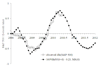
Figure 4 depicts the model linking S&P 500 to the number of 9-year-old, N9. The future numbers of N9 are represented by the number of 3-year-olds, N3, shifted six years ahead. All in all, the level of S&P 500 should suffer a further fall into 2011.

We will be reporting the comparison of the observed and predicted S&P 500 in due course.

Figure 1. Monthly S&P 500 returns

Figure 2. Observed yearly S&P 500 returns and those predicted from real GDP according to the relationship shown in the low left corner of the panel.

Figure 3. Same as in Figure 2 since January 2009.

Figure 4. Observed yearly S&P 500 returns and those predicted from the number of 3-year-olds (at a six year horizon). The relationship is presented in the Figure. In June, the S&P 500 index show fall by another 46 points.

Open new web-site with predicted stock prices

We are opening a new web-site to provide the most recent predictions of (monthly closing) stock prices, infation rate and the long-term forecast of prices of main commodities: oil, gold, metals, grain, etc.

This blog is a very good place for the development and illustration of new ideas. However, the blog format does not allow prompt presenetation of big data sets like the predictions of stock prices of S&P 500 companies. The newly opened web-site will serve as a resource of data and publications, but we will continue review data and the performance of our models in this blog.

So, please visit our web-site: Stock Market Science

CXO and S&P 500 returns

I appreciate the reader's interest to our recent paper "S&P 500 returns revisited" , which resulted in the review made by CXO experts. I have no specific comments on the review except mainly qualitative charater of the assessment. The paper is chiefly quantitative, however.

In this sense, no words can justify our statements, only observations. A year ago, we predicted the fall in May 2010. See what will happen next, and lets revisit the CXO assessment in December 2010. If the model is wrong - everybody will see that it is wrong.

S&P 500: decline and fall

A year ago we predicted a kink in the growth of S&P 500 returns in April-May 2010. This prediction is accurate enough with S&P 500 increased with lower increment in April and May 2010 than it was in April and May 2009.

We've just published a paper (S&P 500 returns revisited) on the prediction where we have put the S&P 500 closing level in April 2010 at 1187 (actual was 1186.68). In May 2010, the (monthly closing) index should fall to 1132 and manifest the start of absolute decrease. So, what we have been recently observing was a decline and we will observed the fall, likely extended into 2011.

Relevant data:
stock prices - finance.yahoo
real GDP - Bureau of Economic Analysis
population - Census Bureau

Figure 1. Observed and predicted S&P 500 returns (12-month cumulated). Notice the turn from growth to fall in April-May 2010. The predicted returns are obtained from the model linking S&P 500 to real GDP. See details in the paper cited in the text.

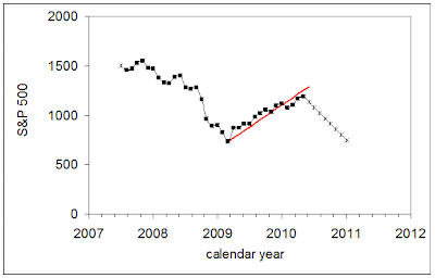
Figure 2. Observed and predicted S&P 500. Red line was predicted in March 2009. The turn in May 2010 is expected with S&P 500 falling from 1187 to 1132. The model links S&P 500 and the number of 9-year-olds, as presented in the paper. According to our estimates, the absolute level of the index may sink below 1000 before 2011 and even 200-250 deeper by July 2011. As before, we display several figures with absolute S&P 500 and its returns.

Figure 3. The prediction of the S&P 500 returns between May 2010 and December 2011. The (12-month cumulated) returns will drop to -0.5. At monthly rates, the returns will be around -0.05 in December 2010.

One may find it interesting to compare our predictions to those made at POLITICAL CALCULATIONS, the only independent blog we have a link to.