Two days ago we revisited share price models for five energy companies from the S&P 500 list: ConocoPhillips (COP), Chevron (CVX), Devon Energy Corporation (DVN), Halliburton (HAL), and Exxon Mobil (XOM). Our pricing model links shares and CPI components (Kitov, 2009). It was demonstrated that all five original models, as had been obtained in 2008, predicted the time history of these prices with a good accuracy. In addition, since the difference between core CPI and headline CPI in the United States is well approximated by a linear function of time this difference can be used to predict share prices in the energy subcategory of the S&P 500 at time horizons of several years.
In this post we are going to improve these models for energy companies using an extended set of 17 individual CPIs, which includes all major subcategories of the headline CPI:
C headline CPI
F food and beverages
H housing
A apparel
T transportation
M medical care
R recreation
ED education
CO communication
O other goods and services
CE CPI less energy
CF CPI less food
CC core CPI
COMM commodities
E energy
NDUR nondurables
CFSHE CPI less food, shelter and energy
This step is in line with our general approach to price modeling, as described by Kitov (2010). We also introduce a quantitative measured of the prediction accuracy – RMSE (root-mean-square error) and check the predictive power of the underlying model.
The pricing model is common for all companies. We assume the presence of a linear link between a share price and the difference between the core (or headline) CPI and some other subset of goods and services comprising the headline CPI. The intuition behind the model is simple; a higher pricing power for a given subcategory of goods and services, and thus related companies, is expressed in a faster increase in corresponding stock prices. In the first approximation, the deviation between relevant price indices is proportional to the ratio of the pricing powers.
The pricing model states that a share price, SP(t), can be approximated by a linear function of the difference between two CPI components, dCPI:
SP(t) = A + B1CPI1(t + t1) + B2CPI2(t + t2) + C(t-t0) (1)
where A, Bi, and C are empirical constants for the studied period (between July 2003 (t0) and November 2010); t is the elapsed time; t1 and t2 are the time delays between the share and the CPIs, both to be determined. Here we introduce a linear trend element, C(t-t0), which has to compensate the trend component in the CPI difference (Kitov&Kitov, 2008). Without loss of generality we minimize the model error by standard LSQ method to find all 6 coefficients (A,Bi,C,ti) for those 2 CPI components among the set of 17, which provide the lowermost RMSE.
Figures 1 and 2 compare two updated predictions for COP and XOM obtained in the previous post with new model based on 17 components. The new models are as follows:
COP(t)= 2.69*H(t+8) – 0.76*T(t+1) – 12.47(t-2000) – 422.1; RMSE=$3.34;
XOM(t)= -2.44*F(t-12) - 1.13*O(t-13) + 31.84(t-2000) + 350.1; RMSE=$4.41
Figure 1. Upper panel: original observed and predicted COP price. A2=72, B2=-5.5 (1999-2009). Lower panel: the improved model described above. The prediction lags by 7 months behind the price.
Figure 2. Same as in Figure 1 for XOM. Original model is characterized by A2=90, B2=-6 (1999-2009).
Figures 3 through 5 compare the original and improved predictions for Chevron, Devon Energy, and Halliburton:
CVX = -5.5*(cCPI - CPI) +85; 1999-2009
CVX(t)= 3.16*H(t) – 10.51*R(t) – 0.90(t-2000) – 565; RMSE=$4.90;
DVN = -7.7*(cCPI - CPI) +97; 1999-2009
DVN(t)= 2.15*CF(t+1) – 0.50*E(t) – 9.72(t-2000) – 304.8; RMSE=$5.88;
HAL = -3.5*(cCPI - CPI) + 43; 1999-2009
HAL(t)= 0.40*T(t+1) – 0.90*O(t+6) + 11.64(t-2000) + 44; RMSE=$2.44
Figure 3. The original and improved share price prediction for CVX
Figure 4. The original and improved share price prediction for DVN
Figure 5. The original and improved share price prediction for HAL
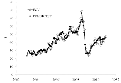
All in all, the extension of the CPI set has significantly improved the predictive power of the model. We have also calculated models for other energy companies. Figure 6 displays two of them:
CHK(t)= -1.47*ED(t-7) + 0.41*E(t+1) +11.4(t-2000) – 12.1; RMSE=$2.68;
ESV(t)= 2.94*C(t) – 2.41*F(t-5) + 2.17(t-2000) – 113; RMSE=$4.14;
Figure 6. Models for CHK and ESV.
References
Kitov, I. (2009). ConocoPhillips and Exxon Mobil stock price, Journal of Applied Research in Finance, v. 2, pp. 129-134.
Kitov, I. (2010). Modelling Share Prices of Banks and Bankrupts, Theoretical and Practical Research in Economic Fields, Association for Sustainable Education, Research and Science, vol. 0(1), pages 59-85, June
Kitov, I., Kitov, O. (2008). Long-Term Linear Trends In Consumer Price Indices, Journal of Applied Economic Sciences, Spiru Haret University, Faculty of Financial Management and Accounting Craiova, vol. 3(2(4)_Summ), pp. 101-112.


No comments:
Post a Comment